TYPICAL components of an INSTRUMENTED GAIT ANALYSIS
The phrase instrumented gait analysis (IGA) is often used to describe the application of computerized measurement technology to clinical gait analysis for the purpose of enhancing the interpretive power of the analysis beyond what can be discerned using observational and physical examination methods alone.
The specialized nature of the systems used to perform an IGA typically requires a dedicated motion laboratory with specialists from clinical and technical disciplines to guide the patient through the testing procedures, make the required physical and anthropometric measurements, and record and process all data (Fig. 16.3). Analyses typically require 2 hours of patient contact time and between 8 and 12 hours of processing and analysis time, depending on the complexity of the patient referral and the number of measurements required to answer the clinical question. It is not within the scope of this discussion to comprehensively describe the full set of measurement tools available for clinical gait analysis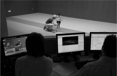
Figure 16.3 A motion laboratory clinical specialist works to place reflective markers on a subject while the technical staff prepares to record data for processing.
in children. For this, the reader is referred to several excellent descriptions that are widely available (5,14,15,16,17,18,19,20). However, since it is important for the discussions that follow, we will briefly introduce the primary measures used, some tips for their practical application, and give examples of typical recordings as a reference.
In addition to the temporal-spatial parameters described in the last section, the primary measurements comprising IGA are gait kinematics, kinetics, and dynamic electromyography (16). While there are certainly additional areas of measurement and many useful instruments that can be included in a comprehensive IGA, these three measurement categories are commonly accepted as the minimum necessary for clinical evaluation of the patient with gait dysfunction, and have been identified by the Commission for Motion Laboratory Accreditation (CMLA) as required for laboratory accreditation (21).
Gait kinematics is a general term that refers to measurement of the linear and angular displacements,
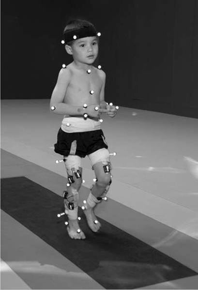
Figure 16.4 Subject with reflective markers or targets placed at strategic anatomic locations walks through a modern motion analysis laboratory. The location of the targets depends on the mathematical requirements of the limb-segment model used to calculate the kinematic values needed for analysis. This subject is using a full body model based on the modified Helen Hayes marker set.
velocities, and accelerations of body segments throughout the gait cycle. Generally expressed in terms of the joint angles between each limb segment, these quantities are most often described three-dimensionally using anatomical planes relative to the more proximal segment, but also includes the global position of the pelvis (pelvic tilt, obliquity, and rotation) and foot (foot progression angle) relative to a fixed laboratory coordinate system located in the middle of the walkway. Modern kinematic analysis systems use an assortment of markers or targets that are attached to the subject at strategic locations and can be tracked by specialized cameras or electromagnetic detectors (Fig. 16.4). The kinematic measurement system identifies the position of the targets from multiple perspectives in three-dimensional space using a high sampling rate (≥100 Hz) as the subject walks through a calibrated measurement volume. This determines a unique trajectory for each target, which can then be reconstructed by the computer utilizing a kinematic link-segment model to produce a three-dimensional animation of the walking subject within the virtual environment of the computer display (Fig. 16.5). From this mathematical representation of the subject, kinematic graphs and interactive reports can be produced to facilitate the clinical analysis of the child's gait pattern.
Kinematic measurement systems rely heavily on motion-capture technology and specialized software that fortunately have found a major market in the video game and motion picture industry.
This has had the positive effect of substantially lowering the startup cost of these systems in recent years, making the technology more available to the clinical community and improving the accuracy, precision, camera resolution, and processing speed. These advances have also increased the complexity of the kinematic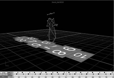
Figure 16.5 Three-dimensional animation of the walking subject within the virtual environment of a computer display.
models that can be implemented, which offers the promise of more comprehensive and anatomically correct descriptions of motion. However, it may also introduce new challenges since increased model complexity necessitates greater software complexity. Furthermore, the requirement for model validation with each new software release necessitates regular laboratory procedural changes, and may introduce data discrepancies when patient results are compared over time using different models. Recognizing these potential technical concerns, gait kinematics represent an integral component of clinical movement analysis and are essential for analyzing the child with gait dysfunction. Figure 16.6 shows a set of three-dimensional kinematic graphs associated with a sample of typically developing 12-13-year-old subjects used as a normal reference in our laboratory. We will discuss
Kinematics Barefoot Walking
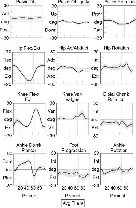
Figure 16.6 Normal three-dimensional kinematic graphs constructed using a sample of typically developing 12- to 13-year-old subjects. These data are used as a reference for comparing kinematic data from clinical subjects. The dark line is the average of all subjects and the gray band represents +/-1 standard deviation.
these kinematic graphs in more detail when discussing critical events in a later section.
While measurements of gait kinematics provide a quantitative description of body segment and joint movement during walking, gait kinetics focus on describing the forces that cause these movements and the calculated quantities that arise when forces and three-dimensional kinematics are combined into a mathematical model of the body.
Since joint and muscle forces cannot be measured directly from the walking subject, the forces due to foot/floor contact are measured using a specialized instrument known as a force platform embedded in the walkway. The force platform measures the vertical, fore-aft shear, and medial-lateral shear components of the ground reaction force (GRF), which is the force vector acting at the supporting surface that is equal and opposite to the sum of all muscular, gravitational, and inertial forces generated by the body in motion. Since a force platform measures the magnitude and direction of the GRF as a single resultant vector quantity, only one foot can be in contact with the platform at a time for a valid measurement. In order to measure multiple foot strikes from both feet, the subject either needs to walk multiple times across a single platform or the laboratory needs to include a force platform array with multiple platforms in different orientations so several clean foot strikes from both sides can be recorded in as few a number of passes as possible. A larger force platform array reduces alterations of gait characteristics in children with neuromuscular diseases in several ways. Installing multiple force platforms into the walkway reduces the number of trials required and thus minimizes the risk of fatigue. Furthermore, having multiple force platforms lessens the possibility of “targeting,” which will alter the subject's characteristic gait pattern. Figure 16.7 shows the large 10-plat- form array of 60 cm ? 40 cm force platforms currently used in our laboratory, and illustrates how rotating the long axis of each platform sequentially 90 degrees can accommodate a wide variety of stride lengths and step patterns for children and adults.The direct measurement of the individual force components and the vector sum of the GRFs has historically been used to evaluate gait kinetics and facilitate a more qualitative pre-/postsurgical comparison. The most useful clinical application of gait kinetics, however, is when it is combined with GRF measurement and a kinetic model of the lower extremities to calculate joint kinetics, specifically joint moments and powers (22).
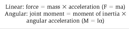
The most common way to accomplish this is to apply an “inverse dynamics” model of the lower extremity using the anthropometric dimensions of each segment (typically seven segments, including the pelvis and both thighs, shanks, and feet) and estimates of each segment's center of mass and inertial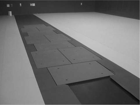
Figure 16.7 Large 10-platform array of 60 cm by 40 cm force platforms used in The Center for Gait and Movement Analysis at The Children’s Hospital in Aurora, Colorado. The “hopscotch” pattern of the platform array permits the recording of several individual foot-strikes from both feet in a single walking pass. For illustration purposes each platform is shown without its protective floor covering, which caused the platforms to blend into the surrounding walkway when applied.
joint is quite useful because the magnitude and sign of the curve at any instance in the cycle can illustrate if one half of the agonist or antagonist pair is dominating at a specific point in the gait cycle. Net moment values can aid in clinical interpretation of gait by comparing them to reference values for typically developing children and by observing changes in the values before and after treatment. In addition, net moment values are helpful in understanding how a child may be compensating at a given joint for weakness or limited range of motion at an adjacent joint. Figure 16.8 shows the sagittal plane kinematics, sagittal plane joint moments, and total joint power for the hip, knee, and ankle from a sample of typically developing 12-13-year-old subjects that we use as a normal reference.
Once the three-dimensional moments at each joint have been calculated, joint power at any time in the gait cycle is the product of the joint moment and the corresponding angular velocity (instantaneous slope of the joint angular displacement curve from kinematics) at each percent interval of the gait cycle:
joint power = joint moment ? joint angular velocity (P(t) = M(t) • ω(t))
quantities. The forces at each joint can then be solved sequentially, starting from the GRF at the floor and working proximally, using the linear and angular forms of Newton's 2nd Law:
By convention, joint moments can be considered either external or internal.
External moments reflect the forces acting on the body through the skeleton that arise from the GRF, and since they reflect an external biomechanical load, are sometimes called demand moments. Internal moments describe the force generated by the muscles and ligaments acting on the skeleton to balance the external moments, and because they are counteracting an external load, are sometimes called response moments. Aside from their different functional descriptions, external and internal moments for the same joint are of equal magnitude and differ only in their mathematical sign. The joint moments described in a typical IGA report are internal moments, but this should always be confirmed since the sign and direction of the curves will be reversed if they actually describe external moments. Joint moments are vector quantities that describe the net torque around each joint but do not provide the individual force contribution from each agonist/antagonist pair or from individual muscles. Nevertheless, the net moment around the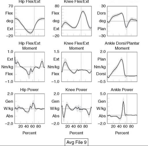
Kinematics and Kinetics: Sagittal
Ankle Dorsi/Plantar
Figure 16.8 Graphs of sagittal plane kinematics, sagittal plane joint moments, and total joint power for the hip, knee and ankle constructed using a sample of typically developing 12- to 13-year-old subjects. These data are used as a reference for comparing kinetic data from clinical subjects. The dark line is the average of all subjects and the gray band represents ± standard deviation.
Just as with joint moments, joint power reflects the net power at a joint and not the individual power generated by a particular muscle or agonist/antagonist pair. However, unlike kinematics and joint moments that simply quantify the motion at a particular instant (kinematics) or calculate an estimate of the force dominating the joint related to muscle function (joint moments), joint power provides insight into the biomechanical mechanisms responsible for specific movements and, in a sense, quantifies the actual “motors” driving a particular gait pattern. In this way, joint power curves are extremely useful to identify when a particular joint is generating power (positive indicates concentric contraction) or absorbing power (negative indicates eccentric contraction) to analyze the transfer of power or energy from one joint to another and for understanding how one joint can compensate for disability at an adjacent joint. It should be pointed out here that although joint power is perhaps the single most informative biomechanical variable that can be obtained from an IGA, it does have limitations (23). For one thing, power is technically a single scalar quantity describing all planes of a joint combined, unlike displacement, velocity, and joint moment, which are directional vector quantities with individual component values for each anatomical plane. While in most cases the greatest contribution can be assumed to arise from the sagittal plane, the lack of a true directional component (especially at the hip) may lead to incomplete clinical interpretations. Another issue is that since extensive use of mathematical modeling is required to arrive at the joint power values, there are numerous assumptions made in the process and great opportunity for errors or artifacts to influence the final curves. These issues should be considered when utilizing any kinetic variable for clinical decision making. However, they should not hinder the use of this information since these estimates cannot be obtained in vivo by any other means and still provide considerable insight into the functional causes of gait abnormalities.
Electromyography is an important tool for evaluation of muscle and neurologic function and is well understood by the pediatric physiatrist. When used in the context of IGA, the purpose is slightly different from the conventional application. The primary objective of EMG in clinical gait analysis is to identify periods of muscle activation during walking so that decisions can be made regarding the appropriateness of muscle timing for agonists pairs as they selectively activate and deactivate during the gait cycle. This is the reason that we refer to this as dynamic electromyography or d-EMG, since the focus is on the phasic response of muscle during walking or some other functional activity. Since the subject won't be in a stationary position for the test, the instruments and technical procedures are also different from conventional diagnostic EMG. Dynamic electromyography requires a bipolar arrangement of electrodes and miniature differential amplifiers with high common mode rejection ratio (CMRR) placed close to the site of the recording to ensure the EMG signal isn't overwhelmed by motion artifact while the subject moves (Fig. 16.9). Differential amplifiers with high CMRR (typically greater than 100) amplify voltage differences between the inputs and reject common voltages that may arise from movement of the electrodes or the soft tissue vibration that occurs with foot contact. Surface electrodes are the most commonly used electrode type for recording d-EMG from the pediatric patient to avoid the emotional trauma and change in gait pattern that indwelling electrodes often cause. Typically, the active portion of each electrode in the bipolar pair should be small and the pair should be placed as close together as possible along the long axis of the muscle (≤1 cm diameter, ≤2 cm separation) to minimize the effect of crosstalk from surrounding muscles. Unfortunately, surface electrodes are only suitable for recording muscle groups that are directly subcutaneous; if there is a need to evaluate deeper muscles individually, fine-wire electrodes made of a bipolar pair of 50-micron platinum wire must be inserted directly into the muscle of interest using a 25-28-gauge needle. When required, this is the most invasive aspect of an IGA, and should be used only when necessary in the pediatric patient and after all other data have been collected, since the level of patient cooperation and the likelihood of a typical gait pattern decrease considerably after a needle stick. In practice, most of the muscles of interest to the pediatric physiatrist can be successfully
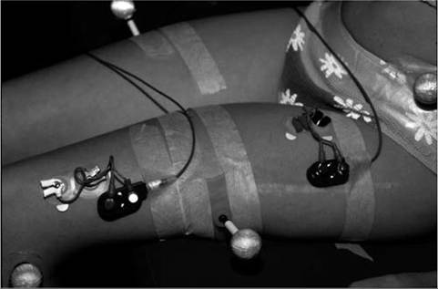
Figure 16.9 Patient with bipolar surface electrodes and small instrumentation amplifiers for recording dynamic EMG while the subject walks. This illustrates the electrode placement for the left vastus lateralis (distal location) and left rectus femoris (proximal location). Each electrode is connected to an instrumented backpack and then hardwired to the recording instruments. A wireless EMG recording system using similar electrodes but with individual transmitters for each muscle is shown in
Figure 16.4. recorded using the surface electrode approach if proper procedures to minimize crosstalk and reduce motion artifact are followed.
Before the EMG recording can be used for clinical interpretation, the raw data must be filtered, processed, and time normalized so periods of muscle activation during the gait cycle can be identified. A good reference for processing guidelines is available from the International Society of Electrophysiology and Kinesiology, where they state that surface electrode recordings should be bandpass-filtered between 10 Hz-350 Hz and fine-wire recordings filtered between 10 Hz-450 Hz. This maximizes the signal, minimizes the noise, and reduces motion artifact. In modern systems, the filtered EMG data are sampled by analog-to-digital converters, and further processing is performed by computer using specialized software or in concert with the motion-capture system. Data can be presented as a continuous recording of “raw” EMG, an ensemble average of several cycles of EMG normalized to the gait cycle, or as linear envelopes reflecting the EMG magnitude throughout the gait cycle after rectification and integration of the raw EMG signal. In our laboratory, we also have developed a system to superimpose the EMG signal over the observational video recording of the walking subject to screen for faulty EMG recording during the analysis and to better understand the interaction between observed movement and muscle activation (see Fig. 16.10, right side). Regardless of how these data are presented, the goal is to use the EMG recording to identify periods of abnormal muscle activity and determine if this activity is responsible for abnormal movement patterns presented by the patient. Typically, the patient's activity is compared
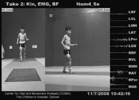
Figure 16.10 Biplane high-definition video recording with superimposed real-time EMG traces of six muscles bilaterally from a typically developing subject used as a reference at CGMA. The raw, unfiltered EMG recording provides immediate feedback on the quality of the EMG signal and the synchronization of muscle activity with observed movement.
to a normal EMG reference, and deviations from normal are scrutinized for their contribution to the overall movement pattern. Figure 16.11 shows filtered and time- normalized EMG for 12 muscles of the lower extremity from a 15-year-old typically developing subject used as a laboratory reference, along with published normal EMG activations represented as solid black bars at the bottom of each graph. The high-magnitude sections of the EMG recording for each muscle correspond to the published normal values, confirming that this typically developing subject has a normal adult activation pattern.
When EMG recordings are combined with the kinematics, kinetics, temporal-spatial parameters, radiographs, and the physical examination results, a comprehensive snapshot of the subject's walking pattern is revealed, providing an empirical basis for identifying the functional cause of a gait abnormality. To use these data successfully, however, we must return to the normal gait cycle to understand the functional requirements for walking, since these requirements are a natural consequence of subdividing the cycle on the basis of function.