Model Description
We developed an agent-based model (ABM) of foraging behavior of the Ache hunters by assuming hunting behavior consistent with Optimal Foraging Theory and based on ecological parameters of the environment and prey characteristics measured in the Mbaracayu Reserve, Paraguay (Janssen and Hill 2014).
Model documentation and code used for this publication can be found at: https://www. openabm.org/model/4538/version/1/view. The Mbaracayu Reserve is part of the traditional foraging territory of the native Ache population whose foraging patterns have been extensively studied from an optimal foraging perspective (e.g. Hawkes et al. 1982; Hill et al. 1987; Kaplan and Hill 1992).The model landscape consists of 58,408 one-hectare cells representing the Mbaracayu Reserve. Each 100 X 100 m cell in the model was assigned a vegetation type based on ground truth transects and subsequent supervised GIS classification with remote sensing using the Landsat 7 TM image with 6 optical bands and one thermal band (Naidoo and Hill 2006). Seven major vegetation habitat types were distinguished: (1) meadow/grassland; (2) large bamboo forest; (3) riparian forest; (4) high forest; (5) low forest; (6) small bamboo understory; and (7) liana forest (Hill et al. 1997). For each hectare cell with an assigned vegetation type, an expected encounter rate for 26 prey types was assigned based on 9 million meters of random diurnal transect monitoring of game encounter rates (Hill et al. 2003; Janssen and Hill 2014).
Our model consists of two types of agents; hunters, and camps, that move on the model landscape. Based on GPS measurements hunters move at a speed of 100 m per 5 min while searching for prey in any of the seven vegetation types. Given the empirically measured mean hunt-day length of 355 min for Ache men (Hill et al. 1985; Hill and Kintigh 2009), hunters can potentially cover on average 7.1 km each day, searching for prey on the simulated landscape.
For each of the 26 prey types in our ABM the following empirically measured characteristics apply: mean live weight of a harvested prey item, mean pursuit time if the prey is hunted upon encounter, and mean probability of a kill (success rate) for all pursuits attempted (see Hill and Kintigh 2009; Janssen and Hill 2014). After the initial assignment of prey densities based on corresponding vegetation types, there are four ways by which prey encounter rates can change through time:
1. Encounter Rate Suppression (ERS). The probability of encountering a prey is reduced for the rest of the day when hunters pass through a cell since they frighten the animals in the cell to hide or move for some time period.
2. Prey Capture (PC). The probability of encountering a prey is adjusted to zero for a cell and some number of surrounding cells whenever a hunt is successful an animal is harvested. The number of cells emptied depends on the density of the species (see Janssen and Hill 2014).
3. Migration (M). Every 3 months there is an update of the prey encounter values by assuming that some animals in nearby cells move into “empty” cells after a conspecific has been harvested. This is an oversimplification adopted for computational reasons, but sensitivity analysis show that more frequent updating does not significantly change the results.
4. Reproduction (R). Once a year we include a reproduction event which follows logistic growth assumptions and increases the probability of encountering prey in cells that were previously emptied after prey harvest.
Each of the 26 prey encounter rates is updated every 5 min in every cell in the model landscape based on ERS and PC. Prey encounter rates are also updated in every cell each three months based on M and once a year due to R.
All hunters live in camps with other hunters, and the location of the next campsite (an agent in the model) often moves each morning (see below). During each 5 min time step through the day, hunters either move/search or hunt/pursue prey without moving.
Hunters are constrained to initially travel in the approximate direction of the campsite for the end of the day (Janssen and Hill 2014).Each time step that a hunter is not in pursuit of a specific prey item, the hunter moves to an adjacent cell and then checks the list of potential prey species in that habitat type in random order to determine whether an encounter takes place in that cell (Fig. 3.1). Prey encounters are assigned probabilistically to match actual measured encounter rates from diurnal transect monitoring. If a prey is encountered, the hunter decides whether to pursue that prey type, and if pursuit is elected, the hunter terminates the probability of encountering any remaining potential prey in that cell. The decision to pursue is based on the expected profitability (kg/h) of the encountered prey type and the mean experienced return rate (kg/h) in the previous 20 days of foraging.
If a hunter is in pursuit during any time step, he remains in pursuit until the assigned prey type pursuit time expires (a defined number of time steps required for each prey
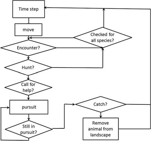
Fig. 3.1 Decision tree for hunters and their related decisions in the agent-based model of foraging
type). If the hunter is not in a pursuit, he checks whether there is still time left in the day to search for prey. If so, the hunter can either turn and move one cell (to repeat the above sequence), or continue moving forward in his previous direction. There is a probability pS that the hunter continues walking straight, and thus a (1-pS) probability that the hunter reorients. As the remaining time left in the day decreases, the hunter becomes more likely to reorient directly towards the next campsite in order to make it to the assigned campsite by the end of the allowed foraging period. Ongoing pursuits continue to termination near the end of the day even if this requires more time than the average assigned foraging day.
In the case of an extra-long foraging day due to pursuit, a new time budget is calculated for the following day that will result in the average hunting time per day of 355 min over the long run.When other hunters are searching nearby, Ache hunters engage in cooperative pursuits for the following species: capuchin monkey, coati, paca, armadillos, and peccaries. Hunters that encounter these prey, often call for others to join a pursuit. Cooperative pursuits increase the total harvest for a band (Hill and Hawkes 1983), but in order for hunters to join in cooperative pursuits, they must move though the landscape in a semi coordinated fashion. In this paper we only include coordinated search with cooperative pursuits for some species. Janssen and Hill (2014) presented analysis of other types of hunter behavior.
The previously published version of the Mbaracayu foraging model allowed us to examine the implications of social living (congregating in camps at the end of each day), cooperative hunting, variation in group size and mobility, under Ache-like ecological conditions. Simulations showed that group living (with presumed sharing) greatly decreased daily risk of no food, but group-based cooperative hunting had only a modest effect of increasing harvest rates. Analysis also showed that bands containing 7-8 hunters that move nearly every day will achieve the best combination of high harvest rates and low probability of no meat in camp (Janssen and Hill 2014). The model predictions of group size, camp mobility, composition of prey harvest, time spent in pursuit, and overall harvest rates corresponded very closely to actual empirically observed patterns by the Ache hunters who live in the study area (Ibid.).
In this paper we extend the prior analysis by exploring the implication how changes in spatial distribution patterns of prey affect optimal camp mobility, camp location and corresponding search patterns by foragers. In the natural Mbaracayu landscape, measured prey encounter rates in each of the seven vegetation habitat types are approximately equal. This probably explains why random walk as a search pattern is such a good null model (Janssen and Hill 2014).
However, most other hunter-gatherer landscapes are likely to be more clumped and patchy, with prey densities that probably vary more between habitat types. How sensitive are the payoffs from Ache-like camp mobility, location and hunting strategies, to landscapes that are more patchy and with higher prey variability across space? To answer this question, we vary the original Ache-like model landscape by modifying the clumpiness of vegetation patterns and the distribution of prey species among vegetation types, while keeping the total prey availability the same. We have chosen to model camp mobility patterns under six alternative habitat conditions: three levels of increasingly clumped habitat types, and two levels of increased variation in prey densities between habitat types (see Table 3.1, Column 1 and Row 1 headings). The model derived from the actual measured Mbaracayu environment we refer to as the “original” environment. It consists of medium clumpiness of vegetation, and low variation in prey biomass between vegetation habitats.3.2.1 Strategies of Camp Movement
In addition to hunters, our models also include mobile agents that represent campsites. The default model behavior that determines the position of a campsite at the end of each day is to randomly relocate the future camp to a spot 2 km from the
Table 3.1 Types of landscapes
| Clumpiness | Original variation in prey biomass | High variation in prey biomass |
| Low | Low | Low |
| Medium | Original | Medium |
| High | High | High |
current camp location each morning. Agents move towards the new camp during the day. This allows us to explore alternative decisions about camp location.
In the targeted campsite version of the model, agents move their camp location into a preferred (high prey density) vegetation type each day.
Agents also keep track where each camp has been and do not reuse old campsites for some time period. The targeted condition constrains the new camp location to cells at least 1 km from a recent campsite. When a camp moves, the nearest vegetation type with the highest return rate which has not been visited during the last 30 days, is the top priority relocation site. This allows foraging agents to spend more time in the highest return vegetation type in an area that has not been recently depleted. If there are no campsites available meeting these criteria, camp will be located in the next highest return vegetation type, and so on, as future campsites are prioritized in descending order of expected foraging return rate in the vegetation habitat where they will be located.When the direction is defined, we will check whether the targeted camp location is between 1 and 3 km. If so, the new camp location will be the target. Otherwise, the camp will move 2 km in the direction earlier defined towards the highest return vegetation type.
The original Ache model specified that camp location always moved after a specified number of days (e.g. one day). In the new adaptive mobility version of the model, the agents residing in a camp together determine whether the average weight of meat hunted over the last few days is above a certain threshold. If so, the camp remains in its location for another day, if not, the campsite is moved to a new location at the beginning of the day.
These two decision criteria define four broad strategies for a camp: whether it is adaptive or not, and whether new locations are targeted or not. This leads to a decision tree on how camps are moved through the landscape (Fig. 3.2).
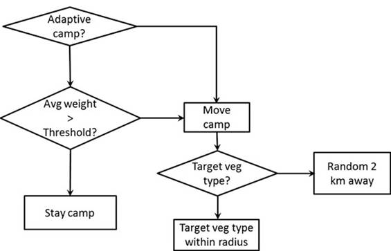
Fig. 3.2 Decision tree for movement of camps including adaptive and targeted movement
Nested within the four camp mobility strategies that we allowed, we can examine several variants. For this paper we varied the threshold for the daily harvest weight that determines whether an adaptive camp stays or moves each day. We explored the threshold values 2, 2.5, 3, 3.5 and 4 kg per hunter per day. We also allowed a range of different group sizes for each camp (1, 2, 3, 4, 5, 6, 7, 8, and 15 hunters) and vary the number of groups to keep the hunting pressure similar. This leads to 108 configurations of camp size and mobility strategies that are imposed on the six different landscape configurations (648 different combinations of camp mobility rules and vegetation habitat configurations).
3.2.2 Alternative Landscapes
In our first publication we examined Ache foraging and camp movement patterns that could maximize foraging gain rates in the actual Mbaracayu environment in which they live. Here we explore optimal strategies when the environment is more clumped and more variable across space. To that end we created alternative resource distributions on the landscape and varied the degree to which vegetation types were more or less productive and the extent to which the cells of different vegetation types were clustered.
The return rates characterizing each of the seven vegetation types are rather equal in the original landscape. Here we amplify the small prey density differences by increasing the encounter rates in the most productive habitat types, and decreasing prey encounter rates in the least productive habitats. Specifically, for the high variation environment we multiplied the prey encounter rates in riparian habitat by 3 and multiplied prey encounter rates in high forest by 2. The remaining 5 vegetation types are multiplied by factors less than one with final prey encounter rates balanced so that the total population of available prey and biomass remains the same over the entire model landscape. Here we assume encounter rate directly relates to the population density of species. This is derived by adjusting the multipliers Mv s such that
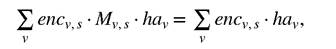
for each species s and where v denotes vegetation type. Encounter rate is defined for each species and vegetation type, encv s and the number of hectares of vegetation type is denoted as hav. Hence if Mv s is increased for two vegetation types, the others will have to be lower than 1 to meet the condition listed above. The multipliers lead to a more unequal distribution of expected return rates for the different vegetation types (Fig. 3.3), with riparian habitat more than ten times as productive as the meadow habitat.
In addition to amplifying the variation or prey densities in habitat types we also modified the landscape by changing the spatial configuration of vegetation types but without changing the total area covered by each habitat type in the model. The natural landscape of the Mbaracayu reserve is composed of multiple habitat types that are distributed in very small patches (often less than 500 m across). To increase the mean size of habitat patches we take the original landscape and perturb this by applying an algorithm which checks if randomly swapping the land cover of two cells leads to a higher degree of similarity between directly neighboring cells. We also applied the inverse algorithm make the landscape more fined grained, with extremely small patches of similar habitat. In the original landscape a one hectare cell has on average 60 % of the cells with the same vegetation type from the 8 neighboring cells that touch it. In our simulations we created artificial landscapes with 30 and 90 % of the neighboring cells containing the same vegetation type (Fig. 3.4).
3.3