Analysis
We ran 64,800 simulations with the Ache model, 100 runs for each of the about 108 configurations on each of the 6 landscapes. Note that we always assume cooperative hunting and coordination between the hunters.
The landscape variants are “original” (O) and “high” (H) variance in prey density across habitats, and “low” (30), “medium” (60), and “high” (90) degrees of clumped habitat.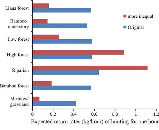
Fig. 3.3 Expected mean return rates on the 7 vegetation types based on prey densities with the original measured values and with the modified encounter rate distribution of higher vegetation variability
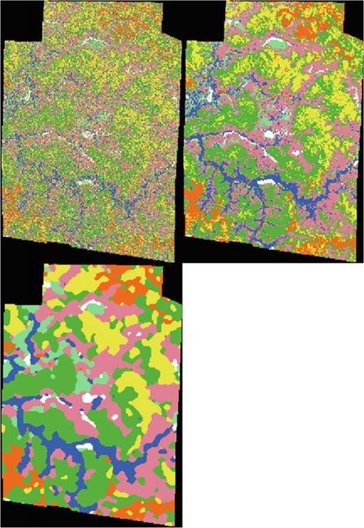
Fig. 3.4 Vegetation maps for less clumped habitat (30), original landscape (60), and more clumped habitat (90) conditions
Figure 3.5 zooms into the results of the targeted movement of the camps. The outcomes of 9 different group sizes are connected to illustrate the effect of group size. Janssen and Hill (2014) used isoclines to find the optimal group size as the combination that leads to high return rates with a low fraction of days without meat. Figure 3.5 shows that for adaptive strategies, the return rates are reduces but the shape is similar.
In Fig. 3.6 we depict for each landscape the results of the 108 camp movement configurations by plotting the average amount of meat per hunter day as well as the
fraction of days that camp residents would consume no meat (because no hunter makes a kill).
Results show that for landscapes with the original measured habitat return rates (O), the best strategy is for groups move each day regardless of clumpedness, and not use an adaptive threshold to determine camp mobility. When the landscape is modified to produce increased variation in return rates among habitat types, the adaptive camp strategy produces increasingly better results than high mobility as the patchiness of the environment increases.
Targeted camp movement is actually worse than random movement when habitats differ little and resources are highly dispersed (O30). When habitats differ little or when habitat types are not clumped, there is no real difference between targeted versus random camp moves. However, when habitat types differ greatly in productivity and when habitats are more clumped in space (H60, H90) substantially greater hunting returns can be obtained by targeting camp moves to prioritize the highest return habitat types.
Without developing a formal model, we presume that foragers prefer both more meat and lower chances of having no game to consume on any given day. In Fig. 3.6 hypothetical isoclines of assumed equal biological utility can be constructed for combinations of return rates and risk of no meat that may be equivalent value to foragers. These isoclines indicate increasing utility to foragers as we move from the lower left to upper right corner in the figure. In all landscapes we find that 7 hunters will maximize the desired combination of higher hunting returns and
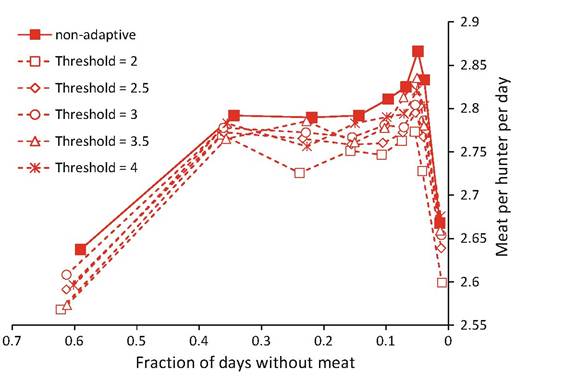
Fig. 3.5 Return rate and days with no meat for 54 permutations of targeted camp movement rules in the original Ache model landscape (O60). Combinations are assumed to have higher biological value moving from lower left to upper right (increasing utility isoclines indicate higher daily return and lower probability of no meat). Camp sizes increase from 1 hunter (far left points) to15 hunters (far right points) for each condition. The optimal combination of high returns and low probability of no-meat is for 7 hunters to move every day (non-adaptive camp mobility)
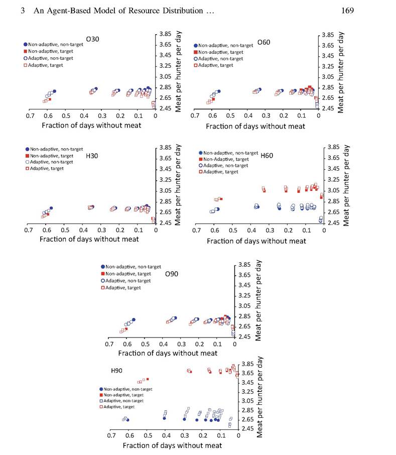
Fig. 3.6 Return rate and days with no meat for 108 permutations of the camp movement rules and in the six different model landscapes described. Combinations are assumed to have higher biological value moving from lower left to upper right (increasing utility isoclines indicate higher daily return and lower probability of no meat) The six figures correspond to the six landscape types defined above (e.g.
O90 = original variation between habitats and highly clumped habitat types). Camp sizes increase from 1 hunter (far left points) to 15 hunters (far right points) for each condition. Adaptive threshold generally decreases in each cluster of unfilled symbols as the y values increase (lower adaptive staying thresholds usually result in higher return rates)lower probability of no meat obtained on single days (see Janssen and Hill 2014). Based on our previous analysis (Ibid.) the optimal group size is found to be a consequence of the advantages of risk reduction with more hunters and the disadvantages of encounter suppression as group size grows. In our simulations, if we reduce the parameter of encounter suppression larger groups are favored, while increasing the impact of encounter suppression reduces the optimal group size. Since we have no empirical measures of this parameter we will stick with our original estimate and for the remainder of this paper we assume a group size of 7 hunters.
We see that for most landscapes the best mobility strategy is for groups to move each day (Table 3.2). Only under high variance in prey density and relatively clumped landscapes does it pay to stay in one camp until daily returns drop below some threshold value. On the other hand, the targeted mobility strategy is more robust, producing higher returns in all environments except those in which habitat types are highly dispersed with little clumping in space. This is because targeted movement allows hunters to spend more time in the best habitat types as long as the camp is located in a reasonable large patch of that habitat type.
In Table 3.3 we present the meat per hunter per day under different conditions and for different mobility strategies. For the adaptive camps we depict the results of the threshold that leads to the best results. We see that the actual Ache mobility pattern (non targeted and non adaptive camp) results in the same food acquisition
Table 3.2 Optimal strategies for different landscapes
| Clumpiness | Original vegetation variability | High vegetation variability |
| Low (30) | Non-targeted camp, non-adaptive camp | Non-targeted camp, non-adaptive camp |
| Original (60) | Targeted camp, non adaptive camp | Targeted camp, adaptive camp. Threshold = 2 kg |
| High (90) | Targeted camp, non-adaptive camp | Targeted camp, adaptive camp. Threshold = 2.5 kg |
Table 3.3 The results for different strategies. For each of the 6 landscapes and each of the four strategies, we provide two numbers: the mean amount of meat per hunter per day (kg/day), and the fraction of days hunters of the camp have not obtained meat from hunting
| Non targeted, non adaptive camp | Non targeted, adaptive camp | Targeted, non-adaptive camp | Targeted, adaptive camp | |
| O30 | 2.850; 0.041 | 2.807; 0.040 | 2.795; 0.050 | 2.764; 0.052 |
| O60 | 2.835; 0.041 | 2.827; 0.047 | 2.866; 0.049 | 2.835; 0.050 |
| O90 | 2.845; 0.041 | 2.803; 0.046 | 2.865; 0.052 | 2.842; 0.054 |
| H30 | 2.785; 0.049 | 2.759; 0.053 | 2.761; 0.055 | 2.757; 0.058 |
| H60 | 2.746; 0.069 | 2.797; 0.067 | 3.115; 0.051 | 3.178; 0.045 |
| H90 | 2.667; 0.125 | 2.876; 0.103 | 3.789; 0.032 | 3.836; 0.026 |
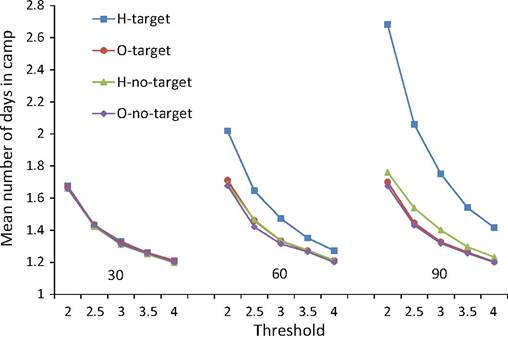
Fig. 3.7 The relationship between the mean number of days adaptive camps remain in the same location on different landscapes, and adopting different mobility thresholds.
Camps are expected to remain longer in one place when resources are more clumped and habitats are more variable (H90) rates on most landscapes, with a slight drop in efficiency on landscapes with more heterogeneity in prey density between habitats. Likewise, on the landscape in which the Ache currently reside (row O60) different mobility strategies lead to very similar results. The strategy Ache hunters use may be the simplest to implement.Figure 3.7 shows that when the landscape is more patchy and clumpy, hunters will achieve higher return rates by camping multiple days in the same camp spot. When the resources on the landscape are more evenly dispersed there is little reason to stay longer in the same location more than one day, and mobility is very high, just as we observe ethnographically among the Ache.
Adopting an adaptive movement strategy or a set mobility interval does not seem to make much difference in our model. This is partially because we have incorporated not cost of camp movement into the model (in both cases men simply hunt along the way to the new campsite). Instead, the key decision in our simulation is when to target specific vegetation types. When two of the vegetation types have much higher return rates and the vegetation types are clustered (H60 and H90) we see major improvement in the overall return rate of hunters when they target certain vegetation types for the location of their camps.
3.4
More on the topic Analysis:
- Analysis of a company’s current financial statements, as described in the Chapters 2 through 4, is enlightening, but not as enlightening as the analysis of its future financial statements.
- Petrographic Analysis
- DATA ANALYSIS
- DATA ANALYSIS
- PROPOSING A COMPREHENSIVE INVESTMENT ANALYSIS METHOD
- Explanatory Analysis of the Model
- TYPICAL components of an INSTRUMENTED GAIT ANALYSIS
- SENSITIVITY ANALYSIS WITH PROJECTED FINANCIAL STATEMENTS
- Legal Analysis
- Analysis of models of competition