Explanatory Analysis of the Model
Below we show the logistic regression analysis on the data from our study in which we set the goal to characterize the abandonment or desertion of a customer from a financial institution starting from a set of explanatory factors.
In this regard, Table 5 displays the first results of the logistic regression analysis.Table 5. Drop-out logistic model: Variables, coefficients and significance (starting solution)
| Variable | β | S.E. | WALD | SIG. | Exp (β) OR |
| ZONE | -0.218 | 0.358 | 0.372 | 0.542 | 0.804 |
| PROD_NUM | 0.108 | 0.098 | 1.236 | 0.266 | 1.115 |
| PROF_RAT | 0.021 | 0.034 | 0.379 | 0.538 | 1.021 |
| RAT_LIQUID | 0.024 | 0.016 | 2.130 | 0.144 | 1.024 |
| PROD_CLASS | -1.410 | 0.672 | 1.266 | 0.260 | 0.244 |
| VOL_CLASS | 0.503 | 0.447 | 4.398 | 0.036(*) | 1.654 |
| RENT_CLASS | -0.484 | 0.489 | 0.981 | 0.322 | 0.616 |
| PAYROLL | -0.173 | 0.404 | 0.183 | 0.669 | 0.841 |
| PENSION | -0.585 | 0.477 | 1.504 | 0.220 | 0.557 |
| DEB_CARD | -0.988 | 0.676 | 2.140 | 0.144 | 0.372 |
| CRED_CARD | 0.641 | 0.372 | 2.969 | 0.085(**) | 1.898 |
| DEBCARD_NUM | 0.904 | 0.307 | 8.652 | 0.003(*) | 2.470 |
| AGE | 0.014 | 0.017 | 0.644 | 0.422 | 1.014 |
| GENDER | -0.560 | 0.401 | 1.954 | 0.162 | 0.571 |
| MOBILE | 0.264 | 0.347 | 0.579 | 0.447 | 1.302 |
| -0.558 | 0.497 | 1.259 | 0.262 | 0.572 | |
| SELF-EMPLOYED | -0.662 | 0.515 | 1.652 | 0.199 | 0.516 |
| YEAS AS A CLIENT | 0.057 | 0.050 | 1.291 | 0.256 | 1.058 |
| E-BANK_NUM | 0.001 | 0.001 | 0.892 | 0.345 | 1.001 |
| E-BANK_AMOUNT | 0.000 | 0.000 | 0.093 | 0.760 | 1.000 |
| CLARITY | 47.134 | 0.000(*) | |||
| (2) | 2.435 | 0.575 | 17.922 | 0.000(*) | 11.418 |
| (3) | 5.246 | 0.770 | 46.457 | 0.000(*) | 189.827 |
| (4) | 2.930 | 1.488 | 3.876 | 0.049(*) | 18.723 |
| (5) | 7.053 | 68.046 | 0.028 | 0.897 | 1156.322 |
| AGILITY | 25.321 | 0.000(*) | |||
| (2) | 1.132 | 0.574 | 3.890 | 0.049(*) | 3.102 |
| (3) | 3.553 | 1.729 | 23.732 | 0.000(*) | 34.931 |
| (4) | 3.956 | 1.177 | 4.322 | 0.009(*) | 52.247 |
| (5) | 6.378 | 15.688 | 0.301 | 0.297 | 588.749 |
| CONFIDENCE | bgcolor=white>5.679 | 0.224 | |||
| (2) | 1.638 | 0.814 | 14.047 | 0.000(*) | 5.144 |
| (3) | 1.459 | 1.205 | 12.4666 | 0.000(*) | 4.300 |
| (4) | 3.454 | 1.960 | 3.104 | 0.038(*) | 31.614 |
| (5) | 5.297 | 15.777 | 0.413 | 0.077(**) | 199.731 |
| SECURITY | 7.214 | 0.125 | |||
| (2) | 0.086 | 2.170 | 0.002 | 0.968 | 1.090 |
| (3) | 2.152 | 1.756 | 1.501 | 0.221 | 8.601 |
| (4) | 2.590 | 1.197 | 4.678 | 0.031(*) | 13.324 |
| (5) | 0.084 | 0.787 | 0.011 | 0.915 | 1.087 |
continued on following page
Table 5.
Continued| Variable | β | S.E. | WALD | SIG. | Exp (β) OR |
| CUSTOMER SERVICE | 47.317 | 0.000(*) | |||
| (2) | 0.691 | 0.719 | 3.925 | 0.021(*) | 1.996 |
| (3) | 1.117 | 1.829 | 2.814 | 0.078(**) | 3.055 |
| (4) | 2.200 | 1.245 | 3.124 | 0.072(**) | 9.022 |
| (5) | 2.766 | 0.669 | 17.075 | 0.000(*) | 15.890 |
| SATISFACTION | 34.017 | 0.000(*) | |||
| (2) | 1.744 | 1.815 | 18.095 | 0.000(*) | 5.711 |
| (3) | 3.582 | 0.731 | 32.459 | 0.000(*) | 35.935 |
| (4) | 4.579 | 3.338 | 6.607 | 0.010(*) | 97.412 |
| (5) | 4.924 | 1.707 | 19.602 | 0.000(*) | 137.643 |
| Constant | -10.686 | 1.911 | 31.281 | 0.000(*) |
Chi-Square: 896.137; d.f.: 44; sign.: 0.000
(*) 5% significance level; (**) 10% significance level
We understand that the design of the model should not conclude at this point, but we have to re-build the model including parameters or variables whose coefficients beta are statistically significant so that it can be possible to transcribe a mathematical equation (terms 3 and 4).
Thus, dating processing obtained from the customer satisfaction survey with the financial institution and its credit history (by binary logistic regression module of SPSS software vs. 20) concludes the final results shown in Table 6.Regarding the evaluation of the model and its coefficients as shown in Table 6, it is appropriate to interpret the influence of the explanatory variables on the dependent variable. Firstly, we emphasize the influence of the customer classification carried out by the financial institution regarding their connection with the volume of business of the institution. According to the way this variable is designed, we accept a positive sign in the estimator or coefficient, as exp (βi) = exp (0.678) = 1.969 is the OR to appear as the
Table 6. Desertion logistic model: Variables, coefficients, and significance (final solution)
| Variable | β | S.E. | WALD | SIG. | Exp (β) OR |
| VOL_CLASS | 0.678 | 0.322 | 4.429 | 0.035(*) | 1.969 |
| CRED_CARD | 0.448 | 0.328 | 3.153 | 0.086(**) | 1.566 |
| DEBCARD_NUM | 0.659 | 0.202 | 10.648 | 0.001(*) | 1.927 |
| CLARITY | 51.545 | 0.000(*) | |||
| (2) | 2.429 | 0.526 | 21.345 | 0.000(*) | 11.350 |
| (3) | 4.910 | 0.695 | 49.938 | 0.000(*) | 135.674 |
| (4) | 3.643 | 1.351 | 7.267 | 0.007(*) | 38.199 |
| (5) | 6.839 | 9.703 | 0.039 | 0.778 | 933.980 |
| AGILITY | 22.933 | 0.000(*) | |||
| (2) | 0.669 | 0.672 | 2.013 | 0.030(*) | 1.952 |
| (3) | 3.000 | 0.651 | 21.250 | 0.000(*) | 20.079 |
| (4) | 3.299 | 2.628 | 4.677 | 0.000(*) | 27.106 |
| (5) | 5.128 | 9.385 | 0.488 | 0.156 | 168.762 |
continued on following page
Table 6.
Continued| Variable | bgcolor=white>βS.E. | WALD | SIG. | Exp (β) OR | |
| CONFIDENCE | 6.363 | 0.182 | |||
| (2) | 1.721 | 0.361 | 22.770 | 0.000(*) | 5.595 |
| (3) | 1.360 | 0.574 | 15.225 | 0.000(*) | 3.898 |
| (4) | 3.9148 | 1.700 | 8.368 | 0.004(*) | 50.320 |
| (5) | 4.974 | 10.960 | 0.740 | 0.076(**) | 144.676 |
| CUSTOMER SERVICE | 50.741 | 0.000(*) | |||
| (2) | 0.423 | 1.645 | 4.431 | 0.011(*) | 1.527 |
| (3) | 0.824 | 1.728 | 3.279 | 0.075(**) | 2.279 |
| (4) | 2.131 | 1.068 | 3.983 | 0.46(*) | 8.8423 |
| (5) | 2.603 | 0.614 | 17.952 | 0.000(*) | 13.498 |
| SATISFACTION | 36.973 | 0.000(*) | |||
| (2) | 1.993 | 1.938 | 20.937 | 0.000(*) | 7.358 |
| (3) | 3.224 | 1.119 | 35.333 | 0.000(*) | 25.133 |
| (4) | 3.992 | 2.812 | 7.760 | 0.005(*) | 54.241 |
| (5) | 4.933 | 1.686 | 20.023 | 0.000(*) | 138.868 |
| Constant | -9.668 | 1.223 | 62.529 | 0.000(*) |
Chi-Square: 696.359; d.f.: 44; sign.: 0.000
(*) 5% significance level; (**) 10% significance level
category “one” instead of “zero.” The estimate indicates that customers with a high turnover with the financial institution are 1,969 times more likely to be loyal than customers with a low turnover.
In the second place, the explanatory model is sensitive to ownership or not of credit cards contracted with the institution with a confidence level of 90%, though. In this case, exp (βi) = exp (0,448) = 1,566 indicates the fact that credit card holders are 1,566 times more likely to remain bank customers and not desert from the financial institution. The next significant characteristic explaining bank loyalty is considered a numeric variable in which exp (βi) = exp (0.659) = 1.927is the OR per debit card hired. That is to say, a person who contracts one more credit card with the financial institution is 1,927 times more likely to be loyal to the institution than the customer who has one less credit card contracted.With respect to categorical variables, the interpretation of the OR for each category cannot be performed independently, but through a comparison with the reference category. In the case of the variable concerning the degree of customer satisfaction with the financial institution as to the clarity of management, the interpretation is as follows: A “very satisfied” customer has an associated probability of being faithful 11,350 times higher than a “dissatisfied” customer.
On the other hand, a “somewhat satisfied” customer is about 135 times more likely to be loyal than a customer who is “dissatisfied” with management clarity, and so on for the categories in which the associated significance level is less than 0.05 or 0.1. With respect to the other categorical variables, the interpretation is similar, keeping in mind that the comparisons are made in relation to the reference category. Likewise, the abovementioned interpretation can be made from an opposite perspective. For example, with respect to the variable SATISFACTION, those overall dissatisfied customers are 54.241 times more likely to drop out than overall satisfied customers.
To sum up, suppose the estimator sign is positive; thus, when the independent variable increases in one unit, the log-odds about the likelihood of being a faithless customer increases in the value of the respective coefficient, and vice-versa for negative estimator.
Therefore, all the independent variables of the final model influence on the behaviour of financial loyalty of each customer, accepting the evidence supported by the research hypotheses H1, H2, H3 and H4.Regarding the goodness of fit, the software calculates coefficients similar to R2 calculated in linear regression, specifically the Cox and Snell R2 and Nagelkerke R2, whose corresponding values (Table 7), point out a good fit in logistic regression.
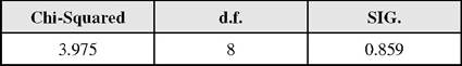
Another source which has been consulted in order to evaluate the goodness of fit of the model is the Hosmer-Lemeshow test. (Table 8), where observations are grouped for each of the two groups defined by the dependent variable depending on a contingency table. The goodness of fit determines the degree of resemblance (adjustment) existing between the observed values and those predicted by the model. It can be seen how the Hosmer- Lemeshow test gives a satisfactory result, given that its significance level is over 5% and cannot, therefore, reject the null hypothesis of equal distributions and, consequently, we can assume that the model provides a good fit to the data.
Table 7. Goodness of fit: Pseudo-R2
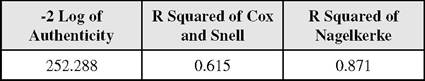
Table 8. Goodness of fit: Hosmer-Lemeshow test
The classification matrix, that is to say, the table of estimated values versus observed values (Table 9), shows the degree of classification accuracy. It can be seen how, for an optimal cut-off point of 0.57, we obtain an accuracy of 94.6% in the correct classification of the borrowers of the database.