Aggregate growth accounting
2.1. The role of information technology
At the aggregate level information technology is identified with the outputs of computers, communications equipment, and software. These products appear in the GDP as investments by businesses, households, and governments along with net exports to the rest of the world.
The GDP also includes the services of IT products consumed by households and governments. A methodology for analyzing economic growth must capture the substitution of IT outputs for other outputs of goods and services.While semiconductor technology is the driving force behind the spread of IT, the impact of the relentless decline in semiconductor prices is transmitted through falling IT prices. Only net exports of semiconductors, defined as the difference between U.S. exports to the rest of the world and U.S. imports appear in the GDP. Sales of semiconductors to domestic manufacturers of IT products are precisely offset by purchases of semiconductors and are excluded from the GDP.
Constant quality price indexes, like those reviewed in the previous section, are a key component of the methodology for analyzing the American growth resurgence. Computer prices were incorporated into the NIPA in 1985 and are now part of the PPI as well. Much more recently, semiconductor prices have been included in the NIPA and the PPI. The official price indexes for communications equipment do not yet reflect the important work of Doms (2004). Unfortunately, evidence on the price of software is seriously incomplete, so that the official price indexes are seriously misleading.
2.1.1. Output
The output data in Table 1 are based on the most recent benchmark revision of the national accounts through 2000.[445] The output concept is similar, but not identical, to the concept of gross domestic product used by the BEA. Both measures include final outputs purchased by businesses, governments, households, and the rest of the world.
Unlike the BEA concept, the output measure in Table 1 also includes imputations for the service flows from durable goods, including IT products, employed in the household and government sectors.The imputations for services of IT equipment are based on the cost of capital for IT described in more detail below. The cost of capital is multiplied by the nominal value of IT capital stock to obtain the imputed service flow from IT products. In the business sector this accrues as capital income to the firms that employ these products as inputs. In the household and government sectors the flow of capital income must be imputed. This same type of imputation is used for housing in the NIPA. The rental value of renter- occupied housing accrues to real estate firms as capital income, while the rental value of owner-occupied housing is imputed to households.
Current dollar GDP in Table 1 is $11.3 trillions in 2002, including imputations, and real output growth averaged 3.46 percent for the period 1948-2002. These magnitudes can be compared to the current dollar value of $10.5 trillions in 2002 and the average real growth rate of 3.36 percent for period 19480-2002 for the official GDP. Table 1 presents the current dollar value and price indexes of the GDP and IT output. This includes outputs of investment goods in the form of computers, software, communications equipment, and non-IT investment goods. It also includes outputs of non-IT consumption goods and services as well as imputed IT capital service flows from households and governments.
The most striking feature of the data in Table 1 is the rapid price decline for computer investment, 15.8 percent per year from 1959 to 1995. Since 1995 this decline has increased to 31.0 percent per year. By contrast the relative price of software has been flat for much of the period and began to fall only in the 1980s. The price of communications equipment behaves similarly to the software price, while the consumption of capital services from computers and software by households and governments shows price declines similar to computer investment.
The top panel of Table 2 summarizes the growth rates of prices and quantities for major output categories for 1989-1995 and 1995-2002. Business investments in computers, software, and communications equipment are the largest categories of IT spending. Households and governments have also spent sizable amounts on computers, software and communications equipment. Figure 1 shows that the share of software output in the GDP is largest, followed by the shares of communications equipment and computers.
20
Table 1
Information technology output and gross domestic product
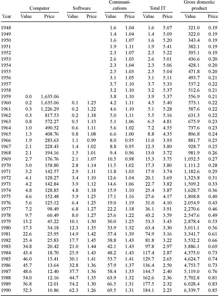
Table 1
(Continued')
| Year | Computer | Software | Communi cations | Total IT | Gross domestic product | |||||
| Value | Price | Value | Price | Value | Price | Value | Price | Value | Price | |
| 1991 | 52.5 | 10.77 | 70.8 | 1.25 | 66.9 | 1.33 | 190.3 | 2.23 | 6,464.4 | 0.87 |
| 1992 | 55.2 | 9.76 | 76.7 | 1.16 | 70.5 | 1.31 | 202.5 | 2.10 | 6,795.0 | 0.89 |
| 1993 | 56.3 | 8.57 | 86.1 | 1.14 | 76.7 | 1.29 | 219.1 | 2.00 | 7,038.5 | 0.89 |
| 1994 | 60.4 | 8.20 | 93.3 | 1.11 | 84.3 | 1.26 | 238.0 | 1.94 | 7,579.6 | 0.93 |
| 1995 | 74.9 | 5.61 | 102.0 | 1.09 | 94.4 | 1.21 | 271.2 | 1.72 | 7,957.1 | 0.95 |
| 1996 | 84.8 | 3.53 | 115.4 | 1.05 | 107.8 | 1.18 | 307.9 | 1.48 | 8,475.5 | 0.97 |
| 1997 | 94.1 | 2.43 | 142.3 | 1.00 | 119.2 | 1.17 | 355.6 | 1.31 | 8,960.9 | 0.98 |
| 1998 | 96.6 | 1.69 | 162.5 | 0.97 | 124.0 | 1.11 | 383.1 | 1.15 | 9,346.9 | 0.98 |
| 1999 | 101.9 | 1.22 | 194.7 | 0.97 | 133.9 | 1.05 | 430.5 | 1.05 | 9,824.2 | 0.98 |
| 2000 | 109.9 | 1.00 | 222.7 | 1.00 | 152.6 | 1.00 | 485.2 | 1.00 | 10,399.5 | 1.00 |
| 2001 | 98.5 | 0.79 | 219.6 | 1.01 | 146.5 | 0.95 | 464.6 | 0.94 | 10,628.5 | 1.01 |
| 2002 | 88.3 | 0.64 | 212.8 | 1.00 | 127.4 | 0.90 | 428.5 | 0.88 | 11,279.4 | 1.04 |
Notes: Values are in billions of current dollars.
Price are normalized to one in 2000. Information technology output is final demand by type of product.2.1.2. Capital services
This section presents capital estimates for the U.S. economy for the period 1948 to 2002.[446] These begin with BEA investment data; the perpetual inventory method generates estimates of capital stocks and these are aggregated, using service prices as weights. This approach, originated by Jorgenson and Zvi Griliches (1967), is based on the identification of service prices with marginal products of different types of capital. The service price estimates incorporate the cost of capital.[447]
The cost of capital is an annualization factor that transforms the price of an asset into the price of the corresponding capital input. This includes the nominal rate of return, the rate of depreciation, and the rate of capital loss due to declining prices. The cost of capital is an essential concept for the economics of information technology,[448] due to the astonishing decline of IT prices given in Tables 1 and 2.
The cost of capital is important in many areas of economics, especially in modeling producer behavior, productivity measurement, and the economics of taxation.[449] Many
Table 2
Growth rates of outputs and inputs
1989-1995 1950-2002
| Prices | Quantiti ( | s Prices | Quantities | |
| Gross domestic product | 2.20 | 2.43 | Outputs 1.39 | 3.59 |
| Information technology | -4.95 | 12.01 | -9.58 | 16.12 |
| Computers | -12.68 | 17.29 | -31.00 | 33.36 |
| Software | -2.82 | 13.35 | -1.31 | 11.82 |
| Communications equipment | -1.36 | 7.19 | -4.16 | 8.44 |
| Non-information technology investment | 2.05 | 1.10 | 2.02 | 2.01 |
| Non-information technology consumption | 2.52 | 2.40 | 1.79 | 3.35 |
| Gross domestic income | 2.45 | 2.17 | Inputs 2.10 | 2.88 |
| Information technology capital services | -3.82 | 12.58 | -10.66 | 18.33 |
| Computer capital services | -10.46 | 20.22 | -26.09 | 32.34 |
| Software capital services | -4.40 | 15.03 | -1.72 | 14.27 |
| Communications equipment capital services | 0.99 | 5.99 | -5.56 | 9.83 |
| Non-information technology capital services | 1.71 | 1.91 | 1.72 | 3.01 |
| Labor services | 3.37 | 1.64 | 3.42 | 1.50 |
The definition of capital includes all tangible assets in the U.S.
economy, equipment and structures, as well as consumers’ and government durables, land, and inventories. The capital service flows from durable goods employed by households and governments enter measures of both output and input. A steadily rising proportion of these service flows are associated with investments in IT. Investments in IT by business, household, and government sectors must be included in the GDP, along with household and government IT capital services, in order to capture the full impact of IT on the U.S. economy.Table 3 gives capital stocks for the business, household and government sectors from 1948 to 2002, as well as price indexes for total domestic tangible assets and IT assets - computers, software, and communications equipment. The estimate of domestic tangible capital stock in Table 3 is $45.9 trillions in 2002, considerably greater than the estimate by BEA. The most important differences reflect the inclusion of inventories and land in Table 3.
Business IT investments, as well as purchases of computers, software, and communications equipment by households and governments, have grown spectacularly in recent years, but remain relatively small. The stocks of all IT assets combined account for only 3.79 percent of domestic tangible capital stock in 2002. Table 4 presents estimates of the flow of capital services from the business, household, and government sectors and corresponding price indexes for 1948-2002.
The difference between growth in capital services and capital stock is the improvement in capital quality. This represents the substitution towards assets with higher marginal products. The shift toward IT increases the quality of capital, since computers, software, and communications equipment have relatively high marginal products. Capital stock estimates fail to account for this increase in quality and substantially underestimate the impact of IT investment on growth.
Table 7 shows the growth of capital quality is near twenty percent of capital input growth for the period 1948-2002.
However, improvements in capital quality have increased steadily in relative importance. These improvements jumped to 46 percent of total growth in capital input during the period 1995-2002, reflecting very rapid restructuring of capital to take advantage of the sharp acceleration in the IT price decline. Capital stock has become progressively less accurate as a measure of capital input and is now seriously deficient.Figure 5 gives the IT capital service flows as a share of gross domestic income. The second panel of Table 2 summarizes the growth rates of prices and quantities of capital inputs for 1989-1995 and 1995-2002. Growth of IT capital services jumps from 12.58 percent per year in 1989-1995 to 18.33 percent in 1995-2002, while growth of nonIT capital services increases from 1.91 percent to 3.01 percent. This reverses the trend toward slower capital growth through 1995.
2.1.3. Labor services
This section presents estimates of labor input for the U.S. economy from 1948 to 2002. These incorporate individual data from the Censuses of Population for 1970, 1980, and
Table 3
Information technology capital stock and domestic tangible assets
| Year | Computer | Software | Communications | Total IT | Total domestic tangible assets | |||||
| Value | Price | Value | Price | Value | Price | Value | Price | Value | Price | |
| 1948 | 4.6 | 0.93 | bgcolor=white>4.61.99 | 754.9 | 0.11 | |||||
| 1949 | 5.7 | 0.93 | 5.7 | 2.00 | 787.1 | 0.11 | ||||
| 1950 | 7.0 | 0.95 | 7.0 | 2.04 | 863.5 | 0.11 | ||||
| 1951 | 8.6 | 0.99 | 8.6 | 2.13 | 990.4 | 0.12 | ||||
| 1952 | 10.0 | 0.96 | 10.0 | 2.05 | 1,066.5 | 0.12 | ||||
| 1953 | 11.5 | 0.92 | 11.5 | 1.97 | 1,136.3 | 0.13 | ||||
| 1954 | 12.9 | 0.93 | 12.9 | 1.99 | 1,187.7 | 0.13 | ||||
| 1955 | 14.3 | 0.92 | 14.3 | 1.98 | 1,279.3 | 0.13 | ||||
| 1956 | 16.4 | 0.94 | 16.4 | 2.01 | 1,417.8 | 0.14 | ||||
| 1957 | 19.4 | 0.98 | 19.4 | 2.10 | 1,516.9 | 0.14 | ||||
| 1958 | 21.1 | 0.98 | 21.1 | 2.11 | 1,586.0 | 0.14 | ||||
| 1959 | 0.2 | 2,389.62 | 0.1 | 1.16 | 23.1 | 0.98 | 23.4 | 2.11 | 1,682.5 | 0.15 |
| 1960 | 0.2 | 2,389.62 | 0.1 | 1.16 | 24.9 | 0.96 | 25.2 | 2.06 | 1,780.8 | 0.15 |
| 1961 | 0.4 | 1,792.22 | 0.3 | 1.14 | 27.1 | 0.94 | 27.8 | 2.02 | 1,881.0 | 0.15 |
| 1962 | 0.5 | 1,194.81 | 0.4 | 1.10 | 29.9 | 0.94 | 30.8 | 2.00 | 2,007.2 | 0.16 |
| 1963 | 1.0 | 836.37 | 0.7 | 1.06 | 32.0 | 0.92 | 33.7 | 1.94 | 2,115.4 | 0.16 |
| 1964 | 1.6 | 716.89 | 1.0 | 1.04 | 34.5 | 0.91 | 37.1 | 1.90 | 2,201.2 | 0.16 |
| 1965 | 2.2 | 597.41 | 1.5 | 1.02 | 37.8 | 0.89 | 41.5 | 1.86 | 2,339.3 | 0.16 |
| 1966 | 2.9 | 414.53 | 2.1 | 0.94 | 42.1 | 0.88 | 47.1 | 1.78 | 2,534.9 | 0.17 |
| 1967 | 3.7 | 333.84 | 2.9 | 0.97 | 47.9 | 0.89 | 54.5 | 1.78 | 2,713.9 | 0.17 |
| 1968 | 4.3 | 283.77 | 3.4 | 0.96 | 54.4 | 0.91 | 62.1 | 1.79 | 3,004.5 | 0.18 |
| 1969 | 5.3 | 258.34 | 4.6 | 1.01 | 61.7 | 0.93 | 71.6 | 1.82 | 3,339.1 | 0.20 |
| 1970 | 6.3 | 232.09 | 6.2 | 1.09 | 70.0 | 0.96 | 82.5 | 1.87 | 3,617.5 | 0.21 |
| 1971 | 6.3 | 176.08 | 7.0 | 1.06 | 77.3 | 0.98 | 90.7 | 1.86 | 3,942.2 | 0.22 |
| 1972 | 7.4 | 142.24 | 8.1 | 1.05 | 85.1 | 1.01 | 100.7 | 1.87 | 4,463.6 | 0.24 |
| 1973 | 8.7 | 134.90 | 9.6 | 1.07 | 93.8 | 1.02 | 112.0 | 1.89 | 5,021.4 | 0.26 |
| 1974 | 9.2 | 110.16 | 11.7 | 1.12 | bgcolor=white>105.81.07 | 126.7 | 1.94 | 5,442.4 | 0.27 | |
| 1975 | 9.8 | 101.69 | 14.4 | 1.19 | 120.6 | 1.14 | 144.8 | 2.06 | 6,242.6 | 0.30 |
| 1976 | 10.5 | 85.07 | 16.3 | 1.19 | 133.0 | 1.18 | 159.7 | 2.09 | 6,795.1 | 0.32 |
| 1977 | 12.5 | 73.95 | 18.1 | 1.21 | 142.2 | 1.16 | 172.8 | 2.04 | 7,602.8 | 0.35 |
| 1978 | 14.2 | 50.03 | 20.4 | 1.21 | 160.3 | 1.19 | 194.9 | 2.03 | 8,701.7 | 0.38 |
| 1979 | 19.4 | 41.48 | 24.5 | 1.24 | 181.8 | 1.22 | 225.8 | 2.05 | 10,049.5 | 0.43 |
| 1980 | 24.4 | 32.35 | 29.6 | 1.29 | 210.4 | 1.28 | 264.4 | 2.09 | 11,426.5 | 0.47 |
| 1981 | 33.9 | 28.42 | 36.2 | 1.35 | 243.3 | 1.36 | 313.5 | 2.17 | 13,057.6 | 0.53 |
| 1982 | 42.7 | 25.37 | 43.2 | 1.39 | 270.5 | 1.40 | 356.4 | 2.20 | 14,020.9 | 0.55 |
| 1983 | 53.0 | 21.01 | 50.3 | 1.38 | 293.2 | 1.41 | 396.5 | 2.16 | 14,589.5 | 0.57 |
| 1984 | 66.7 | 17.08 | 60.1 | 1.37 | 320.5 | 1.42 | 447.3 | 2.11 | 15,901.1 | 0.60 |
| 1985 | 78.3 | 14.59 | 70.5 | 1.36 | 348.1 | 1.42 | 496.9 | 2.05 | 17,616.4 | 0.64 |
| 1986 | 86.8 | 12.46 | 79.3 | 1.31 | 374.1 | 1.40 | 540.2 | 1.96 | 18,912.4 | 0.67 |
| 1987 | 95.0 | 10.66 | 91.2 | 1.31 | 402.8 | 1.39 | 588.9 | 1.91 | 20,263.4 | 0.70 |
| 1988 | 108.3 | 9.90 | 105.4 | 1.30 | 432.8 | 1.37 | 646.4 | 1.87 | 21,932.4 | 0.74 |
| 1989 | 122.4 | 9.27 | 121.9 | 1.25 | 461.6 | 1.36 | 705.9 | 1.83 | 23,678.3 | 0.78 |
Table 3
(Continued')
| Year | Computer | Software | Communications | Total IT | Total domestic tangible assets | |||||
| Value | Price | Value | Price | Value | Price | Value | Price | Value | Price | |
| 1990 | 123.6 | 8.30 | 140.6 | 1.22 | 487.4 | 1.35 | 751.6 | 1.77 | 24,399.0 | 0.79 |
| 1991 | 125.7 | 7.38 | 163.2 | 1.22 | 508.0 | 1.34 | 796.9 | 1.73 | 24,896.3 | 0.79 |
| 1992 | 129.7 | 6.20 | 175.0 | 1.12 | 528.8 | 1.32 | 833.4 | 1.64 | 25,218.3 | 0.79 |
| 1993 | 138.9 | 5.22 | 199.2 | 1.11 | 550.6 | 1.30 | 888.7 | 1.58 | 25,732.9 | 0.79 |
| 1994 | 155.5 | 4.59 | 218.2 | 1.08 | 578.0 | 1.28 | 951.7 | 1.52 | 26,404.2 | 0.79 |
| 1995 | 178.3 | 3.80 | 242.7 | 1.07 | 605.5 | 1.24 | 1,026.5 | 1.44 | 28,003.7 | 0.82 |
| 1996 | 192.5 | 2.85 | 269.7 | 1.04 | 637.5 | 1.20 | 1,099.7 | 1.34 | 29,246.9 | 0.83 |
| 1997 | 212.5 | 2.15 | 312.3 | 1.00 | 678.7 | bgcolor=white>1.181,203.5 | 1.25 | 31,146.2 | 0.86 | |
| 1998 | 227.4 | 1.55 | 360.6 | 0.97 | 704.3 | 1.11 | 1,292.2 | 1.13 | 33,888.6 | 0.91 |
| 1999 | 252.1 | 1.18 | 433.6 | 0.97 | 741.3 | 1.05 | 1,427.1 | 1.05 | 36,307.5 | 0.95 |
| 2000 | 288.2 | 1.00 | 515.5 | 1.00 | 805.2 | 1.00 | 1,608.9 | 1.00 | 39,597.1 | 1.00 |
| 2001 | 279.5 | 0.80 | 563.7 | 1.01 | 844.3 | 0.95 | 1,687.5 | 0.94 | 42,566.9 | 1.05 |
| 2002 | 281.8 | 0.67 | 583.9 | 1.00 | 874.0 | 0.91 | 1,739.7 | 0.89 | 45,892.1 | 1.11 |
Notes: Values are in billions of current dollars. Price are normalized to one in 2000. Domestic tangible assets include fixed assets and consumer durable goods, land, and inventories.
1990, as well as the annual Current Population Surveys. Constant quality indexes for the price and quantity of labor input account for the heterogeneity of the workforce across sex, employment class, age, and education levels. This follows the approach of Jorgenson, Gollop, and Fraumeni (1987).[450]
The distinction between labor input and labor hours is analogous to the distinction between capital services and capital stock. The growth in labor quality is the difference between the growth in labor input and hours worked. Labor quality reflects the substitution of workers with high marginal products for those with low marginal products. Table 5 presents estimates of labor input, hours worked, and labor quality.
The value of labor expenditures in Table 5 is $6.6 trillions in 2002, 58.3 percent of the value of output. This share accurately reflects the concept of gross domestic income, including imputations for the value of capital services in household and government sectors. As shown in Table 7, the growth rate of labor input decelerated to 1.50 percent for 1995-2002 from 1.64 percent for 1989-1995. Growth in hours worked rose from 1.02 percent for 1989-1995 to 1.16 percent for 1995-2002 as labor force participation increased and unemployment rates declined.
The growth of labor quality has declined considerably since 1995, dropping from 0.61 percent for 1989-1995 to 0.33 percent for 1995-2002. This slowdown captures well- known demographic trends in the composition of the work force, as well as exhaustion
Table 4
Information technology capital services and gross domestic income
| Year | Computer | Software | Communications | Total IT | Gross domestic income | |||||
| Value | Price | Value | Price | Value | Price | Value | Price | Value | Price | |
| 1948 | 1.7 | 1.21 | 1.7 | 8.44 | 321.0 | 0.14 | ||||
| 1949 | 1.4 | 0.87 | 1.4 | 6.12 | 322.0 | 0.13 | ||||
| 1950 | 1.7 | 0.86 | 1.7 | 6.04 | 343.4 | 0.14 | ||||
| 1951 | 2.0 | 0.91 | 2.0 | 6.36 | 382.1 | 0.14 | ||||
| 1952 | 2.6 | 0.97 | 2.6 | 6.78 | 395.1 | 0.14 | ||||
| 1953 | 3.1 | 0.98 | 3.1 | 6.85 | 436.6 | 0.15 | ||||
| 1954 | 2.5 | 0.70 | 2.5 | 4.88 | 428.1 | 0.15 | ||||
| 1955 | 3.5 | 0.87 | 3.5 | 6.08 | 471.8 | 0.16 | ||||
| 1956 | 4.0 | 0.89 | 4.0 | 6.24 | 493.7 | 0.16 | ||||
| 1957 | 3.5 | 0.69 | 3.5 | 4.84 | 537.2 | 0.17 | ||||
| 1958 | 3.9 | 0.70 | 3.9 | 4.88 | 512.6 | 0.16 | ||||
| 1959 | 0.2 | 1,842.99 | 0.1 | 1.54 | 4.9 | 0.81 | 5.2 | 5.66 | 556.9 | 0.17 |
| 1960 | 0.2 | 1,801.00 | 0.1 | 1.51 | 5.1 | 0.76 | 5.3 | 5.33 | 573.1 | bgcolor=white>0.17|
| 1961 | 0.3 | 2,651.34 | 0.1 | 1.53 | 5.3 | 0.72 | 5.7 | 5.15 | 587.6 | 0.17 |
| 1962 | 0.5 | 2,221.36 | 0.2 | 1.59 | 6.3 | 0.77 | 7.0 | 5.41 | 631.3 | 0.18 |
| 1963 | 0.7 | 1,301.75 | 0.3 | 1.40 | 6.2 | 0.68 | 7.1 | 4.63 | 675.9 | 0.19 |
| 1964 | 0.8 | 749.35 | 0.4 | 1.32 | 6.8 | 0.69 | 7.9 | 4.40 | 737.6 | 0.20 |
| 1965 | 1.2 | 680.70 | 0.6 | 1.36 | 8.7 | 0.80 | 10.5 | 4.96 | 806.8 | 0.21 |
| 1966 | 2.2 | 675.44 | 0.9 | 1.43 | 9.2 | 0.75 | 12.4 | 4.73 | 881.7 | 0.22 |
| 1967 | 2.4 | 424.81 | 1.1 | 1.14 | 9.4 | 0.68 | 12.8 | 3.96 | 928.7 | 0.22 |
| 1968 | 2.6 | 329.85 | 1.5 | 1.27 | 9.8 | 0.64 | 14.0 | 3.66 | 981.9 | 0.22 |
| 1969 | 2.7 | 253.51 | 1.7 | 1.11 | 10.9 | 0.64 | 15.3 | 3.44 | 1,052.5 | 0.23 |
| 1970 | 3.6 | 246.32 | 2.3 | 1.17 | 12.7 | 0.68 | 18.5 | 3.58 | 1,111.2 | 0.24 |
| 1971 | 5.2 | 274.21 | 3.5 | 1.52 | 14.3 | 0.70 | 23.0 | 3.87 | 1,182.6 | 0.26 |
| 1972 | 4.9 | 182.44 | 3.7 | 1.37 | 16.0 | 0.73 | 24.5 | 3.58 | 1,323.8 | 0.28 |
| 1973 | 4.4 | 124.14 | 4.2 | 1.32 | 21.7 | 0.92 | 30.2 | 3.91 | 1,509.2 | 0.30 |
| 1974 | 6.6 | 145.93 | 4.9 | 1.34 | 19.5 | 0.76 | 30.9 | 3.56 | 1,628.7 | 0.32 |
| 1975 | 5.9 | 107.43 | 6.2 | 1.46 | 22.3 | 0.82 | 34.4 | 3.56 | 1,808.8 | 0.36 |
| 1976 | 6.6 | 97.74 | 7.0 | 1.44 | 23.9 | 0.82 | 37.5 | 3.51 | 2,054.9 | 0.39 |
| 1977 | 7.0 | 78.00 | 7.7 | 1.43 | 39.4 | 1.26 | 54.2 | 4.54 | 2,270.6 | 0.42 |
| 1978 | 11.8 | 84.61 | 9.0 | 1.50 | 33.6 | 0.98 | 54.4 | 3.92 | 2,547.6 | 0.45 |
| 1979 | 11.6 | 50.14 | 10.4 | 1.50 | 44.9 | 1.19 | 66.8 | 4.00 | 2,878.4 | 0.49 |
| 1980 | 16.6 | 44.40 | 12.2 | 1.51 | 40.0 | 0.96 | 68.8 | 3.41 | 3,011.1 | 0.51 |
| 1981 | 17.6 | 29.68 | 13.7 | 1.45 | 38.6 | 0.84 | 69.9 | 2.84 | 3,341.7 | 0.55 |
| 1982 | 19.7 | 22.39 | 15.2 | 1.39 | 41.4 | 0.83 | 76.3 | 2.61 | 3,532.2 | 0.58 |
| 1983 | 26.6 | 20.57 | 18.0 | 1.40 | 46.4 | 0.87 | 91.1 | 2.61 | 3,886.1 | 0.64 |
| 1984 | 36.5 | 18.42 | 22.4 | 1.46 | 53.9 | 0.93 | 112.8 | 2.64 | 4,375.0 | 0.68 |
| 1985 | 40.0 | 14.01 | 26.7 | 1.46 | 60.3 | 0.96 | 127.0 | 2.45 | 4,624.7 | 0.69 |
| 1986 | 43.6 | 11.46 | 31.0 | bgcolor=white>1.4467.3 | 0.98 | 141.9 | 2.32 | 4,753.7 | 0.70 | |
| 1987 | 54.0 | 11.00 | 36.5 | 1.46 | 78.8 | 1.06 | 169.3 | 2.38 | 5,119.0 | 0.72 |
| 1988 | 53.4 | 8.69 | 44.6 | 1.54 | 97.2 | 1.20 | 195.2 | 2.39 | 5,702.8 | 0.77 |
| 1989 | 58.6 | 7.83 | 54.3 | 1.57 | 98.8 | 1.14 | 211.6 | 2.27 | 6,028.4 | 0.79 |
| 1990 | 65.9 | 7.57 | 60.0 | 1.45 | 102.4 | 1.10 | 228.3 | 2.17 | 6,339.7 | 0.81 |
| 1991 | 65.8 | 6.65 | 62.7 | 1.29 | 97.0 | 0.99 | 225.6 | 1.93 | 6,464.4 | 0.82 |
Table 4
(Continued')
| Year | Computer | Software | Communications | Total IT | Gross domestic income | |||||
| Value | Price | Value | Price | Value | Price | Value | Price | Value | Price | |
| 1992 | 73.2 | 6.22 | 82.4 | 1.45 | 105.4 | 1.02 | 261.0 | 1.99 | 6,795.0 | 0.85 |
| 1993 | 79.4 | 5.38 | 80.0 | 1.21 | 118.1 | 1.09 | 277.5 | 1.85 | 7,038.5 | 0.86 |
| 1994 | 84.0 | 4.46 | 97.3 | 1.29 | 132.6 | 1.14 | 313.8 | 1.83 | 7,579.6 | 0.90 |
| 1995 | 105.2 | 4.18 | 102.7 | 1.21 | 150.2 | 1.20 | 358.0 | 1.80 | 7,957.1 | 0.91 |
| 1996 | 133.1 | 3.73 | 116.3 | 1.20 | 144.2 | 1.07 | 393.5 | 1.66 | 8,475.5 | 0.94 |
| 1997 | 144.0 | 2.77 | 134.4 | 1.17 | 147.6 | 1.01 | 425.9 | 1.46 | 8,960.9 | 0.96 |
| 1998 | 162.4 | 2.12 | 152.5 | 1.10 | 184.4 | 1.15 | 499.3 | 1.37 | 9,346.9 | 0.96 |
| 1999 | 166.5 | 1.48 | 165.7 | 1.00 | 188.1 | 1.06 | 520.2 | 1.15 | 9,824.2 | 0.98 |
| 2000 | 156.9 | 1.00 | 193.8 | 1.00 | 201.4 | 1.00 | 552.1 | 1.00 | 10,399.5 | 1.00 |
| 2001 | 175.6 | 0.88 | 219.0 | 1.01 | 199.5 | 0.88 | 594.1 | 0.92 | 10,628.5 | 1.00 |
| 2002 | 162.9 | 0.67 | 247.2 | 1.07 | 202.4 | 0.82 | 612.5 | 0.86 | 11,279.4 | 1.06 |
Notes: Values are in billions of current dollars. Prices are normalized to one in 2000.
of the pool of available workers. Growth in hours worked does not capture these changes in labor quality growth and is a seriously misleading measure of labor input.
2.2. The American growth resurgence
The American economy has undergone a remarkable resurgence since the mid-1990s with accelerating growth in output, labor productivity, and total factor productivity. The purpose of this section is to quantify the sources of growth for 1948-2002 and various sub-periods. An important objective is to account for the sharp acceleration in the growth rate since 1995 and, in particular, to document the role of information technology.
The appropriate framework for analyzing the impact of information technology is the production possibility frontier, giving outputs of IT investment goods as well as inputs of IT capital services. An important advantage of this framework is that prices of IT outputs and inputs are linked through the price of IT capital services. This framework successfully captures the substitutions among outputs and inputs in response to the rapid deployment of IT. It also encompasses costs of adjustment, while allowing financial markets to be modeled independently.
As a consequence of the swift advance of information technology, a number of the most familiar concepts in growth economics have been superseded. The aggregate production function heads this list. Capital stock as a measure of capital input is no longer adequate to capture the rising importance of IT. A stock measure completely obscures the restructuring of capital input that is such an important wellspring of the growth resurgence. Finally, hours worked must be replaced as a measure of labor input.
Table 5
Labor services
| Year | Labor services | Employment | Weekly hours | Hourly compensation | rowspan=2 bgcolor=white>Hours worked||||
| Price | Quantity | Value | Quality | |||||
| 1948 | 0.06 | 2,324.8 | 150.1 | 0.73 | 61,536 | 40.6 | 1.2 | 129,846 |
| 1949 | 0.07 | 2,262.8 | 165.5 | 0.73 | 60,437 | 40.2 | 1.3 | 126,384 |
| 1950 | 0.08 | 2,350.6 | 181.3 | 0.75 | 62,424 | 39.8 | 1.4 | 129,201 |
| 1951 | 0.08 | 2,531.5 | 210.7 | 0.76 | 66,169 | 39.7 | 1.5 | 136,433 |
| 1952 | 0.09 | 2,598.2 | 222.5 | 0.77 | 67,407 | 39.2 | 1.6 | 137,525 |
| 1953 | 0.09 | 2,653.0 | 238.5 | 0.79 | 68,471 | 38.8 | 1.7 | 138,134 |
| 1954 | 0.09 | 2,588.7 | 240.7 | 0.79 | 66,843 | 38.4 | 1.8 | 133,612 |
| 1955 | 0.09 | 2,675.7 | 252.7 | 0.80 | 68,367 | 38.7 | 1.8 | 137,594 |
| 1956 | 0.10 | 2,738.0 | 272.4 | 0.80 | 69,968 | 38.4 | 1.9 | 139,758 |
| 1957 | 0.11 | 2,740.9 | 293.0 | 0.81 | 70,262 | 37.9 | 2.1 | 138,543 |
| 1958 | 0.12 | 2,671.8 | 307.4 | 0.82 | 68,578 | 37.6 | 2.3 | 134,068 |
| 1959 | 0.11 | 2,762.8 | 316.9 | 0.82 | 70,149 | 37.8 | 2.3 | 137,800 |
| 1960 | 0.12 | 2,806.6 | 341.7 | 0.83 | 71,128 | 37.6 | 2.5 | 139,150 |
| 1961 | 0.12 | 2,843.4 | 352.1 | 0.84 | 71,183 | 37.4 | 2.5 | 138,493 |
| 1962 | 0.13 | 2,944.4 | 374.1 | 0.85 | 72,673 | 37.4 | 2.6 | 141,258 |
| 1963 | 0.13 | 2,982.3 | 382.7 | 0.86 | 73,413 | 37.3 | 2.7 | 142,414 |
| 1964 | 0.13 | 3,055.7 | 412.0 | 0.86 | 74,990 | 37.2 | 2.8 | 144,920 |
| 1965 | 0.14 | 3,149.7 | 448.1 | 0.86 | 77,239 | 37.2 | 3.0 | 149,378 |
| 1966 | 0.15 | 3,278.8 | 494.8 | 0.87 | 80,802 | 36.8 | 3.2 | 154,795 |
| 1967 | 0.16 | 3,327.2 | 518.9 | 0.87 | 82,645 | 36.3 | 3.3 | 156,016 |
| 1968 | 0.17 | 3,405.4 | 582.6 | 0.88 | 84,733 | 36.0 | 3.7 | 158,604 |
| 1969 | 0.18 | 3,491.1 | 641.4 | 0.88 | 87,071 | 35.9 | 3.9 | 162,414 |
| 1970 | 0.20 | 3,439.2 | 683.1 | 0.88 | 86,867 | 35.3 | 4.3 | 159,644 |
| 1971 | 0.22 | 3,439.5 | 740.7 | 0.89 | 86,715 | 35.2 | 4.7 | 158,943 |
| 1972 | 0.23 | 3,528.8 | 813.3 | 0.89 | 88,838 | 35.3 | 5.0 | 162,890 |
| 1973 | 0.25 | 3,672.4 | 903.9 | 0.89 | 92,542 | 35.2 | 5.3 | 169,329 |
| 1974 | 0.27 | 3,660.9 | 979.2 | 0.89 | 94,121 | 34.5 | 5.8 | 168,800 |
| 1975 | 0.29 | 3,606.4 | 1,055.2 | 0.90 | 92,575 | 34.2 | 6.4 | 164,460 |
| 1976 | 0.32 | 3,708.0 | 1,182.6 | 0.90 | 94,922 | 34.2 | 7.0 | 168,722 |
| 1977 | 0.34 | 3,829.8 | 1,321.1 | 0.90 | bgcolor=white>98,20234.1 | 7.6 | 174,265 | |
| 1978 | 0.37 | 3,994.9 | 1,496.8 | 0.90 | 102,931 | 34.0 | 8.2 | 181,976 |
| 1979 | 0.40 | 4,122.6 | 1,660.4 | 0.90 | 106,463 | 33.9 | 8.9 | 187,589 |
| 1980 | 0.44 | 4,105.6 | 1,809.7 | 0.90 | 107,061 | 33.4 | 9.7 | 186,202 |
| 1981 | 0.47 | 4,147.7 | 1,934.6 | 0.91 | 108,050 | 33.3 | 10.4 | 186,887 |
| 1982 | 0.50 | 4,110.2 | 2,056.5 | 0.92 | 106,749 | 33.1 | 11.2 | 183,599 |
| 1983 | 0.54 | 4,172.3 | 2,234.7 | 0.92 | 107,810 | 33.2 | 12.0 | 186,175 |
| 1984 | 0.56 | 4,417.4 | 2,458.3 | 0.93 | 112,604 | 33.3 | 12.6 | 195,221 |
| 1985 | 0.58 | 4,531.7 | 2,646.2 | 0.93 | 115,201 | 33.3 | 13.3 | 199,424 |
| 1986 | 0.64 | 4,567.5 | 2,904.1 | 0.93 | 117,158 | 33.0 | 14.4 | 200,998 |
| 1987 | 0.64 | 4,736.5 | 3,017.3 | 0.94 | 120,456 | 33.1 | 14.6 | 207,119 |
| 1988 | 0.65 | 4,888.8 | 3,173.3 | 0.94 | 123,916 | 33.0 | 14.9 | 212,882 |
| 1989 | 0.68 | 5,051.3 | 3,452.4 | 0.95 | 126,743 | 33.2 | 15.8 | 218,811 |
| 1990 | 0.71 | 5,137.6 | 3,673.2 | 0.96 | 128,290 | 33.0 | 16.7 | 220,475 |
| 1991 | 0.75 | 5,086.7 | 3,806.3 | 0.96 | 127,022 | 32.7 | 17.6 | 216,281 |
Table 5
(Continued')
| Year | Labor services | Employment | Weekly hours | Hourly compensation | Hours worked | |||
| Price | Quantity | Value | Quality | |||||
| 1992 | 0.80 | 5,105.9 | 4,087.4 | 0.97 | 127,100 | 32.8 | 18.8 | 216,873 |
| 1993 | 0.82 | 5,267.6 | 4,323.8 | 0.97 | 129,556 | 32.9 | 19.5 | 221,699 |
| 1994 | 0.83 | 5,418.2 | 4,472.4 | 0.98 | 132,459 | 33.0 | 19.7 | 227,345 |
| 1995 | 0.84 | 5,573.2 | 4,661.5 | 0.98 | 135,297 | 33.1 | 20.0 | 232,675 |
| 1996 | 0.86 | 5,683.6 | 4,878.5 | 0.99 | 137,571 | 33.0 | 20.7 | 235,859 |
| 1997 | 0.89 | 5,843.3 | 5,186.5 | 0.99 | 140,432 | 33.2 | 21.4 | 242,242 |
| 1998 | 0.92 | 6,020.8 | 5,519.5 | 0.99 | 143,557 | 33.3 | 22.2 | 248,610 |
| 1999 | 0.96 | 6,152.1 | 5,908.2 | 1.00 | 146,468 | 33.3 | 23.3 | 253,276 |
| 2000 | 1.00 | 6,268.5 | 6,268.5 | 1.00 | 149,364 | 33.1 | 24.4 | 257,048 |
| 2001 | 1.05 | 6,250.6 | 6,537.4 | 1.00 | 149,020 | 32.9 | 25.6 | 255,054 |
| 2002 | 1.06 | 6,188.7 | 6,576.2 | 1.01 | 147,721 | 32.9 | 26.1 | 252,399 |
Notes: Value is in billions of current dollars. Quantity is in billions of 2000 dollars. Price and quality are normalized to one in 2000. Employment is in thousands of workers. Weekly hours is hours per worker, divided by 52. Hourly compensation is in current dollars. Hours worked are in millions of hours.
2.2.1. Production possibility frontier
The production possibility frontier describes efficient combinations of outputs and inputs for the economy as a whole. Aggregate output Y consists of outputs of investment goods and consumption goods. These outputs are produced from aggregate input X, consisting of capital services and labor services.
Productivity is a “Hicks-neutral” augmentation of aggregate input. The production possibility frontier takes the form:

where the outputs include non-IT output goods Yn and output of computers Yc, software Ys, and communications equipment Ym. Inputs include non-IT capital services Kn and the services of computers Kc, software Ks, and telecommunications equipment Km, as well as labor input L.29 Total factor productivity is denoted by A.
The most important advantage of the production possibility frontier is the explicit role that it provides for constant quality prices of IT products. These are used as deflators for nominal expenditures on IT investments to obtain the quantities of IT outputs. Investments in IT are cumulated into stocks of IT capital. The flow of IT capital services is an aggregate of these stocks with service prices as weights. Similarly, constant quality prices of IT capital services are used in deflating the nominal values of consumption of these services.
29
Services of durable goods to governments and households are included in both inputs and outputs.
Another important advantage of the production possibility frontier is the incorporation of costs of adjustment. For example, an increase in the output of IT investment goods requires foregoing part of the output of consumption goods and non-IT investment goods, so that adjusting the rate of investment in IT is costly. However, costs of adjustment are external to the producing unit and are fully reflected in IT prices. These prices incorporate forward-looking expectations of the future prices of IT capital services.
The aggregate production function employed, for example, by SimonKuznets (1971) and Robert Solow (1957, 1960, 1970) and, more recently, by Jeremy Greenwood, Zvi Hercowitz and Per Krusell (1997, 2000), Hercowitz (1998), and Arnold Harberger (1998) is a competing methodology. The production function gives a single output as a function of capital and labor inputs. There is no role for separate prices of investment and consumption goods and, hence, no place for constant quality IT price indexes for outputs of IT investment goods.
Another limitation of the aggregate production function is that it fails to incorporate costs of adjustment. Robert Lucas (1967) presented a production model with internal costs of adjustment. Fumio Hayashi (2000) shows how to identify these adjustment costs from James Tobin’s (1969) Q-ratio, the ratio of the stock market value of the producing unit to the market value of the unit’s assets. Implementation of this approach requires simultaneous modeling of production and asset valuation. If costs of adjustment are external, as in the production possibility frontier, asset valuation can be modeled separately from production.30
2.2.2. Sources of growth
Under the assumption that product and factor markets are competitive producer equilibrium implies that the share-weighted growth of outputs is the sum of the share-weighted growth of inputs and growth in total factor productivity:
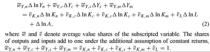
The growth rate of output is a weighted average of growth rates of investment and consumption goods outputs. The contribution of each output is its weighted growth rate. Similarly, the growth rate of input is a weighted average of growth rates of capital and labor services and the contribution of each input is its weighted growth rate. The contribution of total factor productivity, the growth rate of the augmentation.
30
See, for example, John Campbell and Robert Shiller (1998).
Table 6
Sources of gross domestic product growth
| 1948-02 | 1948-73 | 1973-89 | 1989-95 1995-02 | ||
| Gross domestic product | 3.46 | 3.99 | Outputs 2.97 | 2.43 | 3.59 |
| Contribution of information technology | 0.28 | 0.11 | 0.35 | 0.37 | 0.64 |
| Computers | 0.13 | 0.03 | 0.18 | 0.15 | 0.34 |
| Software | 0.07 | 0.02 | 0.08 | 0.15 | 0.19 |
| Communications equipment | 0.08 | 0.07 | 0.09 | 0.08 | 0.11 |
| Contribution of non-information technology | 3.18 | 3.88 | 2.62 | 2.05 | 2.95 |
| Contribution of non-information technology investment | 0.69 | 1.05 | 0.44 | 0.21 | 0.41 |
| Contribution of non-information technology consumption | 2.49 | 2.82 | 2.18 | 1.85 | 2.54 |
| Gross domestic income | 2.79 | 2.99 | Inputs 2.68 | 2.17 | 2.88 |
| Contribution of information technology capital services | 0.36 | 0.15 | 0.38 | 0.49 | 0.93 |
| Computers | 0.17 | 0.04 | 0.20 | 0.22 | 0.52 |
| Software | 0.08 | 0.02 | 0.07 | 0.16 | 0.23 |
| Communications equipment | 0.11 | 0.09 | 0.11 | 0.10 | 0.18 |
| Contribution of non-information technology capital services | 1.39 | 1.79 | 1.15 | 0.71 | 1.07 |
| Contribution of labor services | 1.05 | 1.04 | 1.15 | 0.98 | 0.88 |
| Total factor productivity | 0.67 | 1.00 | 0.29 | 0.26 | 0.71 |
Notes: Average annual percentage rates of growth. The contribution of an output or input is the rate of growth, multiplied by the average value share.
Table 6 presents results of a growth accounting decomposition for the period 19482002 and various sub-periods, following Jorgenson and Stiroh (1999,2000b). Economic growth is broken down by output and input categories, quantifying the contribution of information technology to outputs, as well as capital inputs. These estimates identify computer hardware, software, and communications equipment as distinct types of information technology.
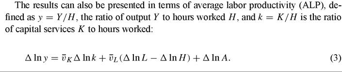
This equation allocates ALP growth among three sources. The first is capital deepening, the growth in capital input per hour worked, and reflects the capital-labor substitution. The second is improvement in labor quality and captures the rising proportion of hours by workers with higher marginal products. The third is total factor productivity growth, which contributes point-for-point to ALP growth. Table 7 shows these estimates.
Table 7
Sources of average labor productivity growth
| 1948-02 | 1948-73 | 1973-89 | 1989-95 | 1995-02 | |
| Gross domestic product | 3.46 | 3.99 | 2.97 | 2.43 | 3.59 |
| Hours worked | 1.23 | 1.06 | 1.60 | 1.02 | 1.16 |
| Average labor productivity | 2.23 | 2.93 | 1.36 | 1.40 | 2.43 |
| Contribution of capital deepening | 1.23 | 1.49 | 0.85 | 0.78 | 1.52 |
| Information technology | 0.33 | 0.14 | 0.34 | 0.44 | 0.88 |
| Non-information technology | 0.90 | 1.35 | 0.51 | 0.34 | 0.64 |
| Contribution of labor quality | 0.33 | 0.43 | 0.23 | 0.36 | 0.20 |
| Total factor productivity | 0.67 | 1.00 | 0.29 | 0.26 | 0.71 |
| Information technology | 0.17 | 0.05 | 0.20 | 0.23 | 0.47 |
| Non-information technology | 0.50 | 0.95 | 0.09 | 0.03 | 0.24 |
Addendum - Growth rates
| Labor input | 1.81 | 1.83 | 1.99 | 1.64 | 1.50 |
| 0.58 | 0.77 | 0.39 | 0.61 | 0.33 | |
| Capital input | 4.13 | 4.49 | 3.67 | 2.92 | 4.92 |
| Capital stock | 3.29 | 4.13 | 2.77 | 1.93 | 2.66 |
| Capital quality | 0.84 | 0.36 | 0.90 | 0.99 | 2.27 |
Notes: Average annual percentage rates of growth. Contributions are defined in Equation (3).
2.2.3. ContributionsofIToutput
Figure 5 depicts the rapid increase in the importance of IT services, reflecting the accelerating pace of IT price declines. In 1995-2002 the capital service price for computers fell 26.09 percent per year, compared to an increase of 32.34 percent in capital input from computers. While the value of computer services grew, the current dollar value was only 1.44 percent of gross domestic income in 2002.
The rapid accumulation of software appears to have different sources. The price of software services has fallen only 1.72 percent per year for 1995-2002. Nonetheless, firms have been accumulating software very rapidly, with real capital services growing 14.27 percent per year. A possible explanation is that firms respond to computer price declines by investing in complementary inputs like software. However, a more plausible explanation is that the price indexes used to deflate software investment fail to hold quality constant. This leads to an overstatement of inflation and an understatement of growth.
Although the price decline for communications equipment during the period 19952002 is greater than that of software, investment in this equipment is more in line with prices. However, prices of communications equipment also fail to hold quality constant. The technology of switching equipment, for example, is similar to that of computers; investment in this category is deflated by a constant-quality price index developed by BEA. Conventional price deflators are employed for transmission gear, such as fiber-
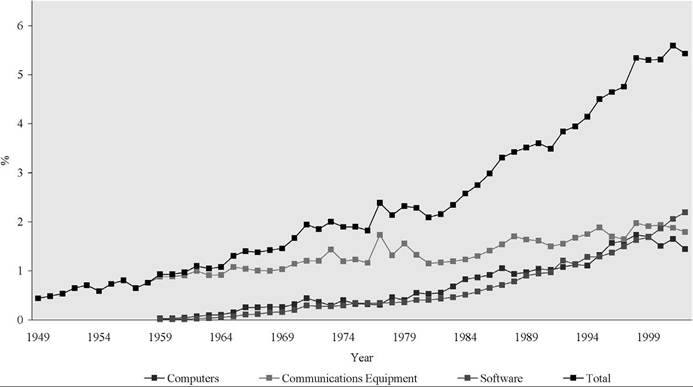
Figure 5. Input shares of information technology by type, 1948-2002. Note: Share of current dollar gross domestic income.
optic cables. This leads to an underestimate of the growth rates of investment, capital stock, capital services, and the GDP, as well as an overestimate of the rate of inflation.
Figures 6 and 7 highlight the rising contributions IT outputs to U.S. economic growth. Figure 6 shows the breakdown between IT and non-IT outputs for sub-periods from 1948 to 2002, while Figure 7 decomposes the contribution of IT into its components. Although the importance of IT has steadily increased, Figure 6 shows that the recent investment and consumption surge nearly doubled the output contribution of IT. Figure 7 shows that computer investment is the largest single IT contributor after 1995, but that investments in software and communications equipment are becoming increasingly important.
Table 2 reports IT input prices and Figures 8 and 9 present a similar decomposition of IT inputs into production. The contribution of these inputs is rising even more dramatically. Figure 8 shows that the contribution of IT now accounts for more than 45.0 percent of the total contribution of capital input. Figure 9 reveals that computer hardware is the largest component of IT, reflecting the growing share and accelerating growth rate of computer investment in the late 1990s.
Private business investment predominates in the output of IT, as shown by Jorgenson and Stiroh (2000b) and Oliner and Sichel (2000).[451] Household purchases of IT equipment are next in importance. Government purchases of IT equipment and net exports of
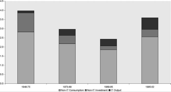
Figure 6. Output contribution of information technology. Note: Output contributions are the average annual growth rates, weighted by the output shares.
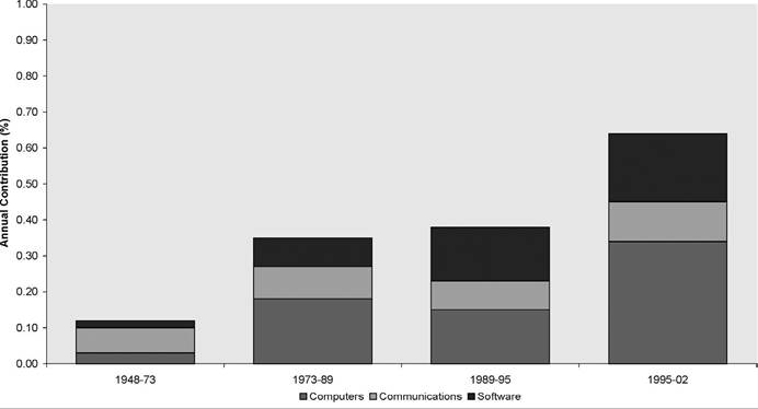
Figure 7. Output contribution of information technology by type. Note: Output contributions are the average annual growth rates, weighted by the output shares.
IT products must be included in order to provide a complete picture. Firms, consumers, governments, and purchasers of U.S. exports are responding to relative price changes, increasing the contributions of computers, software, and communications equipment.
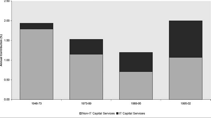
Figure 8. Capital input contribution of information technology. Note: Input contributions are the average annual growth rates, weighted by the income shares.
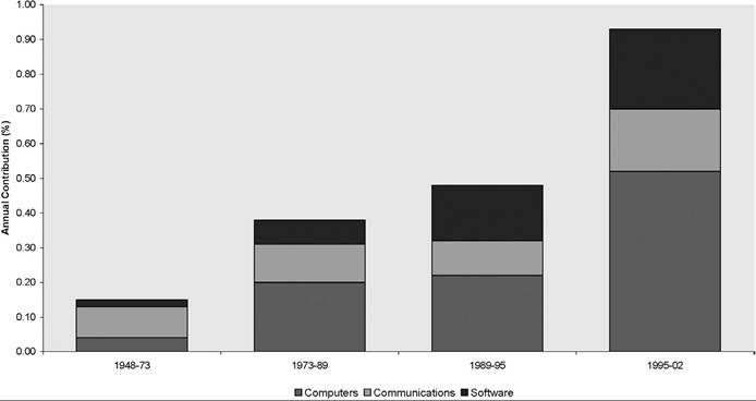
Figure 9. Capital input contribution of information technology by type. Note: Input contributions are the average annual growth rates, weighted by the income shares.
Table 2 shows that the price of computer investment fell by 31.00 percent per year, the price of software fell by 1.31 percent and the price of communications equipment dropped by 4.16 percent during the period 1995-2002, while non-IT investment goods prices rose 2.02 percent. In response to these price changes, firms, households, and governments have accumulated computers, software, and communications equipment much more rapidly than other forms of capital.
2.2.4. Total factor productivity
The price or “dual” approach to productivity measurement employed by Triplett (1996) makes it possible to identify the role of IT production as a source of total factor productivity growth at the industry level.[452] The rate of total factor productivity growth is measured as the decline in the price of output, plus a weighted average of the growth rates of input prices with value shares of the inputs as weights. For the computer industry this expression is dominated by two terms: the decline in the price of computers and the contribution of the price of semiconductors. For the semiconductor industry the expression is dominated by the decline in the price of semiconductors.[453]
Jorgenson, Gollop andFraumeni (1987) have employed Evsey Domar’s (1961) model to trace aggregate productivity growth to its sources at the level of individual in- dustries.[454] More recently, Harberger (1998), William Gullickson and Michael Harper (1999), and Jorgenson and Stiroh (2000a, 2000b) have used the model for similar purposes. Total factor productivity growth for each industry is weighted by the ratio of the gross output of the industry to GDP to estimate the industry contribution to aggregate productivity growth.
If semiconductor output were only used to produce computers, then its contribution to computer industry productivity growth, weighted by computer industry output, would precisely offset its independent contribution to the growth of aggregate productivity. This is the ratio of the value of semiconductor output to GDP, multiplied by the rate of semiconductor price decline. In fact, semiconductors are used to produce telecommunications equipment and many other products. However, the value of semiconductor output is dominated by inputs into IT production.
The Domar aggregation formula can be approximated by expressing the declines in prices of computers, communications equipment, and software relative to the price of gross domestic income, an aggregate of the prices of capital and labor services. The rates of relative IT price decline are weighted by ratios of the outputs of IT products to the GDP.
Table 8 reports details of this decomposition of total factor productivity; the IT and non-IT contributions are presented in Figure 10. Production of IT products contributes 0.47 percentage points to total factor productivity growth for 1995-2002, compared to 0.23 percentage points for 1989-1995. This reflects the accelerating decline in relative price changes resulting from shortening the product cycle for semiconductors.
Table 8
Sources of total factor productivity growth
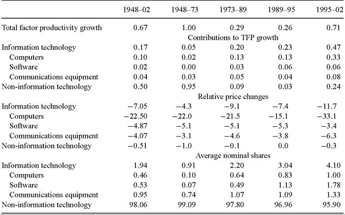
Notes: Average annual rates of growth. Prices are relative to the price of gross domestic income. Contributions are relative price changes, weighted by average nominal output shares.
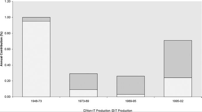
Figure 10. Contribution of information technology to total factor productivity growth. Note: Contributions are average annual relative price changes,weighted by average normal output shares from Table 8.
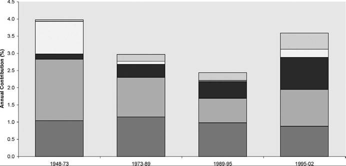
■ Labor Input ? Non-IT Capital Input BIT Capital Input ? Non-IT Production ?IT Production
Figure 11. Sources of gross domestic product growth.
2.2.5. Output growth
This section presents the sources of GDP growth for the entire period 1948 to 2002 as described in Tables 6 and 1. Output grew 3.46 percent per year, as capital services contributed 1.75 percentage points, labor services 1.05 percentage points, and total factor productivity growth only 0.67 percentage points. Input growth is the source of nearly 80.6 percent of U.S. growth over the past half century, while productivity has accounted for 19.4 percent. Figure 11 shows the relatively modest contributions of productivity in all sub-periods.
More than four-fifths of the contribution of capital reflects the accumulation of capital stock, while improvement in the quality of capital accounts for about one-fifth. Similarly, increased labor hours account for 68 percent of labor’s contribution; the remainder is due to improvements in labor quality. Substitutions among capital and labor inputs in response to price changes are essential components of the sources of economic growth.
A look at the U.S. economy before and after 1913 reveals familiar features of the historical record. After strong output and productivity growth in the 1950s, 1960s and early 1910s, the U.S. economy slowed markedly through 1989, with output growth falling from 3.99 percent to 2.91 percent and total factor productivity growth declining from 1.00 percent to 0.29 percent for 1913 to 1989. The contribution of capital input also slowed from 1.94 percent for 1948-1913 to 1.53 percent for 1913-1989. This contributed to sluggish ALP growth-2.93 percent for 1948-1913 compared to 1.36 percent for 1913-1989.
Relative to the period 1989-1995, output growth increased by 1.16 percent during 1995-2002. The contribution of IT production jumped by 0.21 percent, relative to 1989-
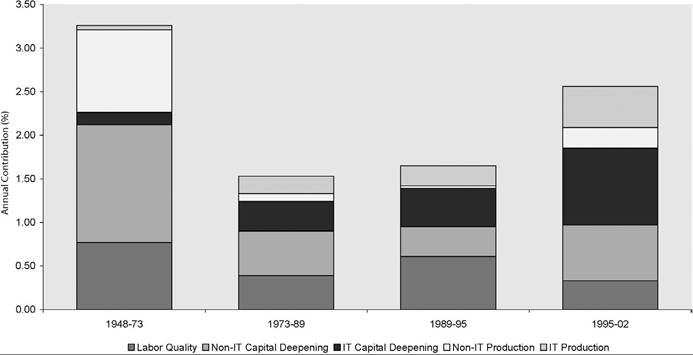
Figure 12. Sources of average labor productivity growth.
1995, but still accounted for only 17.8 percent of the growth of output. Although the contribution of IT has increased steadily throughout the period 1948-2002, there has been a sharp response to the acceleration in the IT price decline in 1995. Nonetheless, more than eighty percent of the output growth can be attributed to non-IT products.
Between 1989-1995 and 1995-2002 the contribution of capital input jumped by 0.80 percentage points, the contribution of labor input declined by 0.10 percent, and total factor productivity accelerated by 0.45 percent. Growth in ALP rose 1.03 percent as more rapid capital deepening and growth in total factor productivity offset slower improvement in labor quality. Growth in hours worked slowed as labor markets tightened considerably, even as labor force participation rates increased.[455]
The contribution of capital input reflects the investment boom of the late 1990s as businesses, households, and governments poured resources into plant and equipment, especially computers, software, and communications equipment. The contribution of capital, predominantly IT, is considerably more important than the contribution of labor. The contribution of IT capital services has grown steadily throughout the period 19482002, but Figure 9 reflects the impact of the accelerating decline in IT prices.
After maintaining an average rate of 0.29 percent for the period 1973-1989, total factor productivity growth declined to 0.26 percent for 1989-1995 and then increased to 0.71 percent peryear for 1995-2002. This is an increasing source of growth in output and ALP for the U.S. economy (Figures 11 and 12). Total factor productivity growth for 1995-2002 is still below the rate of 1948-1973 and the U.S. economy is recuperating from the anemic productivity growth of the past two decades. Slightly more than half of the acceleration in productivity from 1989-1995 to 1995-2002 can be attributed to IT production, which is far greater than the 5.01 percent share of IT in the GDP in 2002.
2.2.6. Average labor productivity
Output growth is the sum of growth in hours and average labor productivity. Table 7 shows the breakdown between growth in hours and ALP for the same periods as in Table 6. For the period 1948-2002, ALP growth predominated in output growth, increasing 2.23 percent per year, while hours worked increased 1.23 percent per year. As shown above, ALP growth depends on capital deepening, a labor quality effect, and overall productivity growth.
Figure 12 reveals the well-known productivity slowdown of the 1970s and 1980s, emphasizing the sharp acceleration in labor productivity growth in the late 1990s. The slowdown through 1989 reflects reduced capital deepening, declining labor quality growth, and decelerating growth in total factor productivity. The growth of ALP recovered slightly during the early 1990s with a slump in capital deepening more than offset by a revival in labor quality growth. A slowdown in hours combined with middling ALP growth during 1989-1995 to produce a further slide in the growth of output. In previous cyclical recoveries during the postwar period, output growth accelerated during the recovery, powered by more rapid growth of hours and ALP.
Accelerating output growth during 1995-2002 reflects modest growth in labor hours and a sharp increase in ALP growth.[456] Comparing 1989-1995 to 1995-2002, the rate of output growth jumped by 1.16 percent - due to an increase in hours worked of 0.14 percent and an upward bound in ALP growth of 1.03 percent. Figure 12 shows the acceleration in ALP growth is due to capital deepening as well as faster total factor productivity growth. Capital deepening contributed 0.74 percentage points to the change, counterbalancing a negative contribution of labor quality of 0.16 percent. The acceleration in total factor productivity growth added 0.45 percentage points.
2.2.7. Research opportunities
The use of computers, software, and communications equipment must be carefully distinguished from the production of IT.[457] Massive increases in computing power, like those experienced by the U.S. economy, have two effects on growth. First, as IT producers become more efficient, more IT equipment and software is produced from the same inputs. This raises total factor productivity in IT-producing industries and contributes to productivity growth for the economy as a whole. Labor productivity also grows at both industry and aggregate levels.
Second, investment in information technology leads to growth of productive capacity in IT-using industries. Since labor is working with more and better equipment, this increases ALP through capital deepening. If the contributions to aggregate output are captured by capital deepening, aggregate total factor productivity growth is unaffected.[458] Increasing deployment of IT affects productivity growth only if there are spillovers from IT-producing industries to IT-using industries.
Jorgenson, Ho and Stiroh (2004) trace the increase in aggregate productivity growth to its sources in individual industries. Jorgenson and Stiroh (2000a, 2000b) present the appropriate methodology and preliminary results. Stiroh (2002) shows that aggregate ALP growth can be attributed to productivity growth in IT-producing and IT-using industries.
2.3. Demise of traditional growth accounting
2.3.1. Introduction
The early 19T0s marked the emergence of a rare professional consensus on economic growth, articulated in two strikingly dissimilar books. Kuznets summarized his decades of empirical research in Economic Growth of Nations (19T1).[459] Solow’s book Economic Growth (19TO), modestly subtitled “An Exposition”, contained his 1969 Radcliffe Lectures at the University of Warwick. In these lectures Solow also summarized decades of theoretical research, initiated by the work of Roy Harrod (1939) and Domar (1946).[460]
Let me first consider the indubitable strengths of the perspective on growth that emerged victorious over its many competitors in the early 19TOs. Solow’s neo-classical theory of economic growth, especially his analysis of steady states with constant rates of growth, provided conceptual clarity and sophistication. Kuznets generated persuasive empirical support by quantifying the long sweep of historical experience of the United States and thirteen other developed economies. He combined this with quantitative comparisons among a developed and developing economies during the postwar period.
With the benefit of hindsight the most obvious deficiency of the traditional framework of Kuznets and Solow was the lack of a clear connection between the theoretical and the empirical components. This lacuna can be seen most starkly in the total absence of cross references between the key works of these two great economists. Yet they were working on the same topic, within the same framework, at virtually the same time, and in the very same geographical location - Cambridge, Massachusetts!
Searching for analogies to describe this remarkable coincidence of views on growth, we can think of two celestial bodies on different orbits, momentarily coinciding from our earth-bound perspective at a single point in the sky and glowing with dazzling but transitory luminosity. The indelible image of this extraordinary event has been burned into the collective memory of economists, even if the details have long been forgotten. The resulting professional consensus, now obsolete, remained the guiding star for subsequent conceptual development and empirical observation for decades.
2.3.2. Human capital
The initial challenge to the framework of Kuznets and Solow was posed by Denison’s magisterial study, Why Growth Rates Differ (1967). Denison retained NNP as a measure of national product and capital stock as a measure of capital input, adhering to the conventions employed by Kuznets and Solow. Denison’s comparisons among nine industrialized economies over the period 1950-1962 were cited extensively by both Kuznets and Solow.
However, Denison departed from the identification of labor input with hours worked by Kuznets and Solow. He followed his earlier study of U.S. economic growth, The Sources of Economic Growth in the United States and the Alternatives Before Us, published in 1962 [Denison (1962)]. In this study he had constructed constant quality measures of labor input, taking into account differences in the quality of hours worked due to the age, sex, and educational attainment of workers.
Kuznets (1971), recognizing the challenge implicit in Denison’s approach to measuring labor input, presented his own version of Denison’s findings.[461] He carefully purged Denison’s measure of labor input of the effects of changes in educational attainment. Solow, for his part, made extensive references to Denison’s findings on the growth of output and capital stock, but avoided a detailed reference to Denison’s measure of labor input. Solow adhered instead to hours worked (or “man-hours” in the terminology of the early 1970s) as a measure of labor input.[462]
Kuznets showed that.. with one or two exceptions, the contribution of the factor inputs per capita was a minor fraction of the growth rate of per capita product”.[463] For the United States during the period 1929 to 1957, the growth rate of productivity or output per unit of input exceeded the growth rate of output per capita. According to Kuznets’ estimates, the contribution of increases in capital input per capita over this extensive period was negative!
2.3.3. Solow's surprise
The starting point for our discussion of the demise of traditional growth accounting is a notable but neglected article by the great Dutch economist Jan Tinbergen (1959), published in German during World War II. Tinbergen analyzed the sources of U.S. economic growth over the period 1870-1914. He found that efficiency accounted only a little more than a quarter of growth in output, while growth in capital and labor inputs accounted for the remainder. This was precisely the opposite of the conclusion that Kuznets (1971) and Solow (1970) reached almost three decades later!
The notion of efficiency or “total factor productivity” was introduced independently by George Stigler (1947) and became the starting point for a major research program at the National Bureau of Economic Research. This program employed data on output of the U.S. economy from earlier studies by the National Bureau, especially the pioneering estimates of the national product by Kuznets (1961). The input side employed data on capital from Raymond Goldsmith’s (1962) system of national wealth accounts. However, much of the data was generated by John Kendrick (1956, 1961), who employed an explicit system of national production accounts, including measures of output, input, and productivity for national aggregates and individual industries.[464]
The econometric models of Paul Douglas (1948) and Tinbergen were integrated with data from the aggregate production accounts generated by Abramovitz (1956) and Kendrick (1956) in Solow’s justly celebrated 1957 article, “Technical change and the aggregate production function” [Solow (1957)]. Solow identified “technical change” with shifts in the production function. Like Abramovitz, Kendrick, and Kuznets, he attributed almost all of U.S. economic growth to “residual” growth in productivity.[465]
Kuznets’ (1971) international comparisons strongly reinforced the findings of Abra- movitz (1956), Kendrick (1956), and Solow (1957), which were limited to the United States.[466] According to Kuznets, economic growth was largely attributable to the Solow residual between the growth of output and the growth of capital and labor inputs, although he did not use this terminology. Kuznets’ assessment of the significance of his empirical conclusions was unequivocal:
(G)iven the assumptions of the accepted national economic accounting framework, and the basic demographic and institutional processes that control labor supply, capital accumulation, and initial capital-output ratios, this major conclusion - that the distinctive feature of modern economic growth, the high rate of growth of per capita product is for the most part attributable to a high rate of growth in productivity - is inevitable.[467]
The empirical findings summarized by Kuznets have been repeatedly corroborated in investigations that employ the traditional approach to growth accounting. This approach identifies output with real NNP, labor input with hours worked, and capital input with real capital stock.[468] Kuznets (1971) interpreted the Solow residual as due to exogenous technological innovation. This is consistent with Solow’s (1957) identification of the residual with technical change. Successful attempts to provide a more convincing explanation of the Solow residual have led, ultimately, to the demise of the traditional framework.[469]
2.3.4. Radical departure
The most serious challenge to the traditional approach growth accounting was presented in my 1967 paper with Griliches, “The explanation of productivity change” [Jorgenson and Griliches (1967)]. Griliches and I departed far more radically than Denison from the measurement conventions of Kuznets and Solow. We replaced NNP with GNP as a measure of output and introduced constant quality indexes for both capital and labor inputs.
The key idea underlying our constant quality index of labor input, like Denison’s, was to distinguish among different types of labor inputs. We combined hours worked for each type into a constant quality index of labor input, using the index number methodology Griliches (1960) had developed for U.S. agriculture. This considerably broadened the concept of substitution employed by Solow (1957). While he had modeled substitution between capital and labor inputs, Denison, Griliches and I extended the concept of substitution to include different types of labor inputs as well. This altered, irrevocably, the allocation of economic growth between substitution and technical change.[470]
Griliches and I introduced a constant quality index of capital input by distinguishing among types of capital inputs. To combine different types of capital into a constant quality index, we identified the prices of these inputs with rental prices, rather than the asset prices used in measuring capital stock. For this purpose we used a model of capital as a factor of production I had introduced in my 1963 article, “Capital theory and investment behavior” [Jorgenson (1963)]. This made it possible to incorporate differences among depreciation rates on different assets, as well as variations in returns due to the tax treatment of different types of capital income, into our constant quality index of capital input.[471]
Finally, Griliches and I replaced the aggregate production function employed by Denison, Kuznets, and Solow with the production possibility frontier introduced in my 1966 paper, “The embodiment hypothesis” [Jorgenson (1966)]. This allowed for joint production of consumption and investment goods from capital and labor inputs. I had used this approach to generalize Solow’s (1960) concept of embodied technical change, showing that economic growth could be interpreted, equivalently, as “embodied” in investment or “disembodied” in productivity growth. My 1967 paper with Griliches [Jorgenson and Griliches (1967)] removed this indeterminacy by introducing constant quality price indexes for investment goods.[472]
Griliches and I showed that changes in the quality of capital and labor inputs and the quality of investment goods explained most of the Solow residual. We estimated that capital and labor inputs accounted for eighty-five percent of growth during the period 1945-1965, while only fifteen percent could be attributed to productivity growth. Changes in labor quality explained thirteen percent of growth, while changes in capital quality another eleven percent.[473] Improvements in the quality of investment goods enhanced the growth of both investment goods output and capital input; the net contribution was only two percent of growth.[474]
2.3.5. The Rees Report
The demise of the traditional framework for productivity measurement began with the Panel to Review Productivity Statistics of the National Research Council, chaired by Albert Rees. The Rees Report of 1979, Measurement and Interpretation of Productivity, became the cornerstone of a new measurement framework for the official productivity statistics. This was implemented by the Bureau of Labor Statistics (BLS), the U.S. government agency responsible for these statistics.
Under the leadership of Jerome Mark and Edwin Dean the BLS Office of Productivity and Technology undertook the construction of a production account for the U.S. economy with measures of capital and labor inputs and total factor productivity, renamed multifactor productivity.[475] The BLS (1983) framework was based on GNP rather than NNP and included a constant quality index of capital input, displacing two of the key conventions of the traditional framework of Kuznets and Solow.[476]
However, BLS retained hours worked as a measure of labor input until July 11, 1994, when it released a new multifactor productivity measure including a constant quality index of labor input as well. Meanwhile, BEA (1986) had incorporated a constant quality price index for computers into the national accounts - over the strenuous objections of Denison (1989). This index was incorporated into the BLS measure of output, completing the displacement of the traditional framework of economic measurement by the conventions employed in my papers with Griliches.[477]
The official BLS (1994) estimates of multifactor productivity have over-turned the findings of Abramovitz (1956) and Kendrick (1956), as well as those of Kuznets (1971) and Solow (1970). The official statistics have corroborated the findings summarized in my 1990 survey paper, “Productivity and economic growth” [Jorgenson (1990)]. These statistics are now consistent with the original findings of Tinbergen (1959), as well as my paper with Griliches (1967), and the results I have presented in Section 2.2.
The approach to growth accounting presented in my 1987 book with Gollop and Fraumeni and the official statistics on multifactor productivity published by the BLS in 1994 has now been recognized as the international standard. The new framework for productivity measurement is presented in a Manual published by the Organization for Economic Co-Operation and Development (OECD) and written by Schreyer (2001). The expert advisory group for this manual was chaired by Dean, former Associate Commissioner for Productivity at the BLS, and leader of the successful effort to implement the Rees Report (1979).
3.