Asimpleframework
We consider an economy where growth is driven by capital accumulation, although the main argument could easily be adapted to the case of a knowledge-based economy where growth is primarily driven by (long-term) innovative investments.
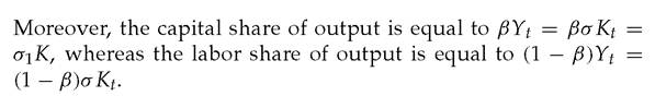
Time is discrete and indexed by t. Labor is supplied inelastically and Lo = 1 is the aggregate labor supply. There is one good in the economy, which is used both for consumption and also as capital input, and is produced according to the standard AK technology: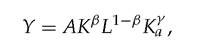
where Ka is the aggregate capital stock and
As in the neoclassical model or the AK model with constant savings rate,3 we assume that all agents consume a fixed fraction α of current period's earnings and save the fixed fraction (1 — α) for investment or lending in the next period.
Using the fact that all firms are identical, we focus on the symmetric equilibrium where they all invest the same amount of capital each period. Then, in equilibrium:
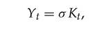
where
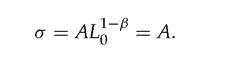
Only firm owners (the capitalists) have access to productive investment opportunities. Workers cannot invest directly in production but they can either lend at the current interest rate r to the borrowers (or entrepreneurs), or invest in a home activity that yields a (low) return rate 
The two key elements of the story we tell in this chapter are credit constraints and price effects.
1.
Credit constraints are modeled as in the previous chapter, by assuming that an entrepreneur with initial wealth W can invest at most μW in the current period. This means that a firm that has a cash flow shock will respond by changing its investment.2. Price effects work through the interest rate which is determined endogenously. The AK nature of the model implies that the equilibrium interest rate will be equal to the rate of return σ1 on capital investment whenever investment demand is higher than aggregate savings, and will drop down to σ2 when investment demand is less than aggregate savings. This in turn affects the ability of the firm to borrow, which affects investment demand, and so on.
The timing of events within each period t is depicted in Figure 3.1.
Borrowing and lending take place at the beginning of the period (which we denote by t-) at an interest rate which is determined as specified above, by the comparison between investment demand and aggregate savings. And everything else happens at the end of the period (which we denote by t+), namely: the realization of returns from investments, the repayment of debt from borrowers to lenders, and finally consumption and savings decisions which in turn determine the total amount of savings available at the beginning of the following period (t + 1)-.
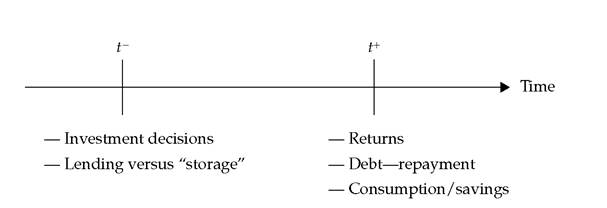
Fig. 3.1 Timing.
Source: Aghion et al. (1999a), figure 1.
3.2