Empiricalanalysis
In the rest of this section we present, based on AABM, some results from trying to test the above predictions.
2.2.1 Data and measurement
Annual growth is computed as the log difference of per capita income obtained from the Penn World Tables (PWT) mark 6.1.
As in Ramey and Ramey (1995), aggregate volatility is measured by taking the country-specific standard deviation of annual growth over the 1960-95 period.Financial development is measured by the ratio of private credit, that is the value of loans by financial intermediaries to the private sector, over GDP. Data for 71 countries on 5-year interval averages between 1960 and 1995 (1960-4, 1965-9, etc.) was first compiled by Levine et al. (2000); an annual dataset was more recently prepared and made available by Levine on his webpage. Private credit is the preferred measure of financial development by Levine et al. because it excludes credit granted to the public sector and funds coming from central or development banks. AABM also conduct sensitivity analysis with two alternative measures of credit constraints: liquid liabilities and bank assets. The first is defined as currency plus demand and interest-bearing liabilities of banks and nonbank financial intermediaries divided by GDP; the second gives the value of all loans by banks but not other financial intermediaries.
The next step in presenting the evidence is to look at the response of growth to specific shocks. AABM first consider terms of trade shocks, available as 5-year averages between 1960 and 1985 from the Barro-Lee (1996) dataset. Changes in the terms of trade reflect export-weighted changes in export prices net of import-weighted changes in import prices, quoted in the same currency. Arguably, exchange rate fluctuations may be endogenous to the growth process and therefore regressions of growth on terms of trade shocks may be subject to reverse causality and produce biased coefficient estimates.
AABM therefore also construct an annual index of export-weighted commodity price shocks using data on the international prices of 42 products between 1960 and 2000 available from the International Financial Statistics (IFS) Database of the IMF.For the analysis on the transmission channel of credit constraints, one also needs data on long-term versus short-run investments. AABM consider R&D as a share of total investment. Unfortunately, data availability limits the sample to 14 OECD countries between 1973 and 1997 for which the OECD reports spending on R&D in the ANBERD database. Data on investment as a share of GDP is easily obtainable from the PWT.
In the growth regressions AABM follow Ramey and Ramey and Levine et al. in controlling for population growth, initial secondary school enrollment, and a set of four policy variables (the share of government in GDP, inflation, the black market exchange rate premium, and openness to trade). We use demographics data from the PWT and the policy conditioning set in Levine et al.
2.2.2 AsummaryoftheAABMresults
While Ramey and Ramey study the response of long-term growth to volatility and Levine et al. focus on the direct effects of credit constraints on growth, our model predicts that volatility is more harmful to long-run growth in financially underdeveloped countries. AABM therefore estimate the basic equation:
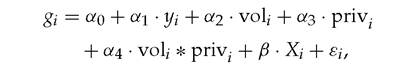
where yi is the initial income in country i, gi denotes the average rate of productivity growth in country i over the whole period 1960-95, voli is the measure of aggregate volatility, privi- is the average measure of financial development over the period 1960-95, Xi is a vector of country-specific controls, and εt is the noise term. We are mostly interested in the interaction term α4 ∙ voli- * privi-, and our first prediction is that α4 should be positive and significant.
We also believe that α2 should be negative and significant, so that volatility is negatively correlated with growth in countries with low financial development, but less so when financial development increases.Table 2.1 presents the results reported in AABM. They find a strong direct negative effect of volatility on long-term growth of -0.41 and a significant positive coefficient on the interaction term of 0.011 (Column (1)). In this sample private credit varies from 4% to 141%, with a mean of 38% and a standard deviation of 29%. A one standard deviation increase in the level of financial development would therefore reduce the impact of a 1% rise in volatility from a 0.41% fall in the growth rate to -0.41 + 0.011 * 29 = -0.09%. This effect is significant in economic terms not only because of the large variation in private credit in the cross-section, but also because of its substantial fluctuations in the time series: For example, in the United States private credit almost tripled between 1960 and 1995, steadily rising from 50% to 140%. For many countries the level of private credit moved up and down significantly during the same period. As Column (2) shows, the AABM result is robust to the inclusion of demographic and human capital controls, as well as measures of property rights protection and the policy variables from Levine et al.
For sufficiently high levels of private credit (which we observe for many OECD countries) these results predict that the overall contribution of volatility to economic growth becomes positive. Moreover, for intermediate levels of private credit the gross contribution may be close to zero. Regressing long-run growth on
Table 2.1 Growth, volatility, and credit constraints: basic specification
No investment
With investment
Whole sample OECD countries Whole sample OECD countries
| Independent variable | (1) | (2) | (3) | (4) | (5) | (6) | (7) | (8) |
| Initial income | -0.0071 | -0.0174 | -0.0177 | -0.0256 | -0.0103 | -0.0159 | -0.0173 | -0.0256 |
| (-2.56)** | (-5.77)*** | (-6.69)*** | (-6.32)*** | (-4.10)*** | (-5.70)*** | (-6.55)*** | (6.01)*** | |
| Volatility | -0.4129 | -0.5098 | -0.5165 | -0.5196 | -0.3012 | -0.4245 | -0.5446 | -0.5607 |
| (-3.06)*** | (-3.33)*** | (-1.73)* | (-1.14) | (-2.52)** | (-2.98)*** | (-1.83)* | (-1.16) | |
| -0.00005 | -0.00016 | -0.00019 | -0.00006 | -0.00008 | -0.00020 | -0.00021 | -0.00008 | |
| (-0.29) | (-0.98) | (-1.26) | (-0.29) | (-0.60) | (-1.34) | (-1.39) | (-0.37) | |
| Volatility* private credit | 0.0113 | 0.0090 | 0.0080 | 0.0040 | 0.0069 | 0.0069 | 0.0083 | 0.0049 |
| (2.59)** | (2.15)** | (1.67)^ | (0.63) | (1.76)* | (1.78)* | (1.73)∧ | (0.72) | |
| Investment/GDP | 0.1420 | 0.0857 | 0.0270 | 0.0218 | ||||
| (4.68)*** | (3.20)*** | (1.13) | (0.63) | |||||
| Pop growth | -0.0081 | 0.0005 | -0.0076 | 0.0018 | ||||
| (-3.55)*** | (0.17) | (-3.64)*** | (0.48) | |||||
| Sec school enrollment | 0.0037 | 0.0064 | -0.0040 | 0.0056 | ||||
| (0.28) | (1.15) | (-0.33) | (0.92) |
| Government size | -0.00001 | 0.00006 | -0.00013 | 0.00027 | ||||
| (-0.04) | (0.14) | (-0.43) | (0.51) | |||||
| Inflation | 0.0003 | -0.0004 | 0.0002 | 0.0001 | ||||
| (2.78)*** | (-0.52) | (1.91)* | (0.11) | |||||
| Black market premium | -0.0072 | -0.0380 | -0.0082 | -0.0218 | ||||
| (0.91) | (-0.34) | (-1.14) | (-0.18) | |||||
| Trade openness | 0.00011 | -0.00004 | 0.00009 | -0.00003 | ||||
| (2.06)** | (-0.62) | (1.98)* | (-0.36) | |||||
| Intell property rights | 0.0013 | -0.0015 | 0.0018 | -0.0007 | ||||
| (0.50) | (-0.50) | (0.76) | (-0.22) | |||||
| Property rights | 0.0023 | 0.0003 | 0.0018 | 0.0009 | ||||
| (1.94)* | (0.23) | (1.64)∧ | (0.57) | |||||
| F-test (volatility terms) | 0.0103 | 0.0051 | 0.2462 | 0.4122 | 0.0489 | 0.0105 | 0.2157 | 0.4580 |
| F-test (credit terms) | 0.0001 | 0.0310 | 0.0690 | 0.3993 | 0.0814 | 0.2120 | 0.1125 | 0.3875 |
| R[5] | 0.3141 | 0.6576 | 0.7894 | 0.9534 | 0.4889 | 0.7212 | 0.8049 | 0.9569 |
| N | 70 | 59 | 22 | 19 | 70 | 59 | 22 | 19 |
Note: Dependent variable is average growth over the 1960-95 period.
All regressors are averages over the 1960-95 period, except for intellectual and property rights which are for 1970-95 and 1970-90 respectively. Initial income and secondary school enrollment are taken for 1960. Constant term not shown. T-statistics in parenthesis. P-values from an F-test of the joint significance of volatility terms (volatility and volatility*credit) and credit terms (credit and volatility*credit) reported. ***, **, *,^significant at the 1%, 5%, 10%, and 11% respectively.volatility alone without accounting for the direct and interacted effects of financial development, could thus produce an insignificant coefficient. This may explain why Ramey and Ramey find a strong negative effect of volatility on growth in the full crosssection but a nonsignificant one in the OECD sample. In Columns (3) and (4) AABM estimate the above equation for the OECD countries only, and find coefficients similar to the ones we find for the entire sample.
Finally, Columns (5) and (6) show that the growth impact of both volatility itself and its interaction with private credit are little affected by the inclusion of investment as a control. Risk arguably affects savings rates and investment, and investments fuel growth. However, controlling for the ratio of investment to GDP reduces the coefficient on volatility by only 20%, suggesting that 80% of the total effect of volatility on growth is via a channel other than the rate of investment.
These results have been shown to be robust to alternative measures of financial development, namely liquid liabilities and bank assets.2
Next, to address the potential endogeneity problem raised by the above measure of volatility, AABM analyze the sensitivity of growth to exogenous shocks, exploring both the cross-section and time-series variation in the panel. They consider average data over 5-year period intervals in a cross-section of over 70 countries to estimate the following specification:
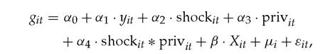
where git and privy are the annual growth and private credit averages for country i in the 5-year subperiod t, and yu is the initial per capita income at the beginning of the subperiod.
To measure the shock term, shockit, we consider both the average terms-of- trade shock and the average commodity price shock during the subperiod. We expect a positive terms-of-trade shock to stimulate growth, and therefore α2 to be positive. Similarly, we anticipate a positive direct effect of financial development, thus α3 shouldTable 2.2 The response of growth to terms of trade and commodity price shocks: 5-year averages
| Independent variable | Terms of trade shocks | Price commodity shocks | ||||||
| Private creditt | Initial credit | Lagged credit | Private creditt | Initial credit | Lagged credit | |||
| OLS (1) | FE (2) | FE (3) | FE (4) | OLS (5) | FE (6) | FE (7) | FE (8) | |
| Initial income | -0.0063 | -0.0757 | -0.0670 | -0.0899 | -0.0076 | -0.0701 | -0.0592 | -0.0751 |
| (-2.02)** | (-8.06)*** | (-7.22)*** | (-7.12)*** | (-2.68)*** | (-8.34)*** | (-6.92)*** | (-7.00)*** | |
| Shock | 0.1402 | 0.1383 | 0.1062 | 0.1640 | 0.1297 | 0.1243 | 0.1462 | 0.1234 |
| (3.07)*** | (3.60)*** | (2.31)** | (3.65)*** | (2.43)** | (2.68)*** | (2.45)** | (2.36)** | |
| Private credit | 0.0143 | 0.0177 | 0.0145 | 0.0264 | 0.0387 | 0.0325 | ||
| (1.71)* | (1.09) | (0.64) | (3.61)*** | (3.21)*** | (1.99)** | |||
| Private credit*shock | -0.3226 | -0.3509 | -0.0539 | -0.3599 | -0.2263 | -0.2119 | -0.4207 | -0.2065 |
| (-1.89)* | (-2.24)** | (-0.23) | (-1.78)* | (-1.22) | (-1.33) | (-1.44) | (-0.99) | |
| Controls | ||||||||
| pop growth, sec enroll | yes | yes | yes | yes | yes | yes | yes | yes |
| R2 | 0.0696 | 0.0867 | ||||||
| R2 within | 0.3296 | 0.3418 | 0.3608 | 0.2723 | 0.2650 | 0.2519 | ||
| R2 between | 0.0419 | 0.0287 | 0.0320 | 0.0403 | 0.0322 | 0.0516 | ||
| # countries (groups) | 73 | 57 | 70 | 72 | 57 | 72 | ||
| N | 323 | 323 | 277 | 255 | 388 | 388 | 331 | 321 |
Note: Dependent variable is average growth over 5-year intervals in the 1960-85 period.
Terms of trade shock is defined as the growth of export prices less the growth of import prices. Commodity price shocks are export-weighted changes in the price of 42 commodities. Both shocks are averaged over the corresponding 5-year interval. Private credit is concurrent 5-year average, initial 1960-64 average or lagged (t-5,t-1) average as indicated in the column heading. Constant term not shown. T-statistics in parenthesis. ***, **, *, ^ significant at the 1%, 5%, 10%, and 11% respectively.
Source: AABM (2004), table 4.
Table 2.3 The response of investment to commodity price shocks: annual panel data, fixed effects
| Dependent variable: Credit and prop rights: Independent variable: | Investment/GDP | R&D/investment | ||||||
| (t-5,t-1) avg | (t-10,t-6) avg | (t-5,t-1) avg | (t-10,t-6) avg | |||||
| (1) | (2) | bgcolor=white>(3)(4) | (5) | (6) | (7) | (8) | ||
| Shockt | -2.56 | -9.19 | -27.60 | -9.14 | 0.2629 | 0.7217 | 0.5945 | 0.2863 |
| (-0.21) | (-0.20) | (-0.59) | (-0.85) | (0.65) | (0.52) | (0.58) | (0.79) | |
| Shockt-1 | 10.06 | 22.58 | 47.85 | 12.61 | 0.0547 | 1.0157 | 0.4940 | 0.0642 |
| (0.82) | (0.47) | (1.00) | (1.16) | (0.14) | (0.70) | (0.48) | (0.18) | |
| Shockt-2 | -7.56 | 111.51 | 148.02 | -13.19 | 0.7429 | -1.0500 | 0.0350 | 0.8298 |
| (-0.65) | (3.09)*** | (3.89)*** | (-1.20) | (1.94)* | (-0.97) | (0.04) | (2.24)** | |
| Priv credit | 1.83 | -0.17 | -1.71 | 5.93 | -0.0583 | 0.0078 | -0.0685 | -0.0735 |
| (1.32) | (-0.11) | (-0.77) | (3.72)*** | (-1.29) | (0.17) | (-1.41) | (-1.37) | |
| Priv credit*shockt | 11.54 | 9.81 | 8.43 | 23.25 | -0.3734 | -0.2190 | -0.2459 | -0.4368 |
| (0.62) | (0.39) | (0.34) | (1.40) | (-0.61) | (-0.29) | (-0.45) | (-0.78) | |
| Priv credit*shockt-1 | -2.23 | 0.14 | -16.62 | -3.42 | -0.0871 | -0.0220 | 0.0518 | -0.1722 |
| (-0.12) | (0.01) | (-0.69) | (-0.20) | (-0.14) | (-0.03) | (0.10) | (-0.30) | |
| Priv credit*shockt-2 | 26.09 | 40.46 | 2.85 | 38.12 | -1.2544 | -1.2025 | -1.1847 | -1.5159 |
| (1.46) | (2.06)** | (0.14) | (2.08) * * | (-2.12) * * | (-2.04)** | (-2.75)*** | (-2.45)** | |
Controls
| Linear trend | Yes | Yes | Yes | Yes | Yes | Yes | Yes | Yes |
| Intell rights + interact | Yes | Yes | Yes | Yes | ||||
| Prop rights + interact | Yes | Yes | ||||||
| R2 within | 0.2535 | 0.2581 | 0.2295 | 0.2848 | 0.5053 | 0.5804 | 0.6228 | 0.5084 |
| R2 between | 0.0519 | 0.1470 | 0.1016 | 0.0635 | 0.2292 | 0.1518 | 0.2325 | 0.2227 |
| # countries (groups) | 14 | 14 | 13 | 14 | 14 | 14 | 13 | 14 |
| N | 337 | 291 | 221 | 331 | 338 | 291 | 221 | 332 |
Note: Dependent variable is investment as a share of GDP or R&D as a share of investment. Annual 1973-97 data, except where lost due to lags. Panel fixed effects estimation. Shockt, shockt-1, shockt-2 refer to the contemporaneous, 1-year and 2-year lagged commodity price shock, as defined in the text. Lagged (t-10,t-6) or (t-5,t-1) average used for private credit, as indicated in the column heading. All regressions include a constant term and a linear trend. T-statistics in parenthesis. ***,**,* significant at the 1%, 5%, and 10% respectively.
Source: AABM (2004), table 7.
also be positive. We are particularly interested by the interaction term α4 ∙ shocki't * privrt and we predict that α4 should be negative, which says that a higher level of financial development will imply a lower sensitivity of growth to shocks. In the estimation we allow for country-specific fixed effects.
Table 2.2 summarizes the results from AABM. In particular, it shows evidence of a significantly positive effect of shocks on medium-run growth. We also observe a strong negative coefficient on the interaction term, although it is only significant when we consider changes in the terms of trade. This result is shown to be robust to alternative measures of financial development and to using a one-period lagged value of private credit. Because of the substantial time-series variation in private credit it is not surprising that using its initial 1960 value produces an insignificant interaction term.
The final link that remains to be established is the interaction of financial development with the cyclicality of long-term investment and total investment with respect to exogenous shocks. As a proxy for long-term investment, AABM use data on R&D expenditures. Using annual data on 14 OECD countries between 1973 and 1997, AABM perform two first-stage regressions, respectively for R&D as a share of total investment (R&Dn/In) and investment as a fraction of GDP (˛ö/GDPn) for country i in year t, as a function of current and lagged shocks and current and lagged shocks (one and two period lags) interacted with private credit in the country during subperiod t. As before, they include a linear trend and allow for country fixed effects.
Table 2.3 displays the results from these two regressions. Column (5) uses the moving average of private credit over the immediately preceding 5 years. In line with the model, we see that positive shocks stimulate R&D for a given level of total investment, but the ratio of R&D over total investment tends to be countercyclical in the absence of credit constraints. In particular, all coefficients on lagged shocks are positive, while the interaction terms of these shocks with private credit have a negative and significant coefficient. Two-year lagged shocks are the only significant ones, suggesting that the reallocation of investment itself takes place with a lag. To gauge the importance of credit constraints, note that R&D is procyclical for low levels of financial development but a value for private credit of 0.74/1.25 = 60% is enough to make long-term investment countercyclical with respect to twice-lagged shocks. In fact, we observe such high levels of loan availability for many countries in our sample of 70, with the number tripling to 36 between 1974 and 1999. These results are shown to be robust to using the 5-year lagged 5-year average of private credit (Columns (6)-(8)).
In contrast to the above findings, the share of total investment in GDP does not become more procyclical as credit constraints tighten (Table 2.3, Columns (1)-(4)). If anything, financial development may magnify the procyclicality of the investment over GDP ratio, if we rely on the only significant (and positive) interaction coefficients in Columns (2) and (4). Overall, these results support our theory that credit availability redirects resources toward longterm projects (such as R&D) during a downturn, translating into improved growth a year or two later.
2.3