Towardamacropolicyofgrowth
In this chapter, we have proposed an explanation for the observed negative correlation between volatility and growth across countries, and also for the fact that the correlation is more significantly negative once we include non-OECD countries in the regressions.
Our explanation combines credit constraints with entrepreneurs' choice between short-term capital and long-term growth-enhancing (R&D) investments. The main predictions from the theory are that in economies with lower levels of financial development: (i) volatility affects growth more negatively; (ii) growth is more sensitive to trade or price commodity shocks; (iii) R&D is more procyclical. As argued in the previous section and in greater detail in AABM, all these predictions are validated by available cross-country panel data on volatility, growth, R&D, and total investments over the period 1960-95.To conclude this chapter, we would like to suggest two directions in which to pursue this research program and exploit our main findings so far. Both avenues have to do with the interplay between macropolicy and long-run growth, a topic on which endogenous growth theory has so far remained relatively silent.[6] The first avenue, currently explored by Aghion-Bacchetta- Ranciere-Rogoff (2004), henceforth ABRR, concerns the relationship between long-run growth and the choice of exchange rate regime. The second avenue, currently explored by Aghion- Barro-Marinescu, henceforth ABM, builds on the analysis in this chapter to revisit budgetary policies and their effects on long-run growth.
2.3.1 Productivity growth and the choice of exchange rate regime
The existing theoretical literature on exchange rates and open macroeconomics does not look at long-run growth, except for few regressions (e.g., by Ghosh et al. 2003) that did not find any systematic relationship between the two.
Based on a variant of the model in this chapter, but with nominal rigidities so that nominal exchange rates can have an impact on real decisions and outcomes, ABRR predict that in economies with lower level of financial development, a flexible exchange rate regime will tend to generate excessive currency appreciations which in turn will make all firms (including the best performing ones) become more vulnerable to other shocks, for example, on the liquidity needs of long-term (productivity-enhancing) investments. This, in turn, will tend to discourage innovative investments.ABRR consider a growing, small open economy with overlapping generations of entrepreneurs and workers. They assume that nominal wages are rigid and that the central bank either fixes the nominal exchange rate or follows an interest rate rule. The model focuses on the interaction of nominal exchange rate fluctuations and productivity growth.
The small open economy produces a single good identical to the world good. At each period a new generation of two-period lived individuals is born. One half of the individuals is selected to become entrepreneurs, while the other half become workers. If entrepreneurs go bankrupt when young, they become workers when old and are replaced by old workers in the firm. Since we abstract from saving and capital accumulation, individuals consume their income each period.
During the first period of their life, entrepreneurs can produce using a technology with current average productivity, namely:
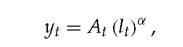
where a < 1 and lt is labor input. At the end of the first period, entrepreneurs can invest in innovation and thereby realize extra rents in their second period. The foreign price of the good is taken as given. Purchasing power parity (PPP) holds so that

where Pt is the domestic price level and St is the nominal exchange rate (domestic per foreign currency).
In a fixed exchange rate, one would set St = S, while under a flexible exchange rate one has E(St) = S. The nominal wage is preset before knowing nominal shocks, but after productivity is known, and it is preset at a level equal to the reservation wage of workers.The entrepreneur chooses lt to maximize ex ante expected profits, which in turn yields an equilibrium expected profit of the form:
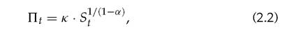
where κ is a constant (see ABRR for details). Thus, more volatile exchange rates translate into more volatile current profits.
Next, ABRR introduce innovation and credit constraints. As in AABM, they assume that an entrepreneur can remain active in the second period of his/her life, and thereby upgrade his/her technology, provided he/she can pay a liquidity cost (or "innovation cost") cl, which in principle differs across firms and must be incurred by each firm at the end of its first period. We assume that the net productivity gain from innovating is sufficiently high that it is profitable for any entrepreneur to invest in innovation.
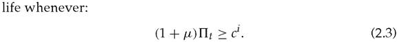
Again, in order to pay for the liquidity cost, the entrepreneur can borrow on the local credit market. However, we assume the existence of credit constraints which prevents him/her from borrowing more than a finite multiple μ∏t of his/her current profits. We take μ as the measure of financial development.
Thus, the funds available for innovative investment at the end of the first period, are at most equal to (1 + μ)∏t and therefore the entrepreneur will continue in the second period of his/her
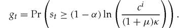
Using (2.2), this gives:

where st = ln St.
Thus, an entrepreneur is more likely to continue when the exchange rate is depreciated and with a large level of financial development. We now turn to the determination of the exchange rate.
ABRR follow AABM in assuming that knowledge At grows at a rate which is proportional to the total number of innovations in the economy, and for notational simplicity let us assume that it is equal to that number. By the law of large numbers the rate of productivity growth is thus simply equal to:
We can now analyze how the average growth rate depends upon the variance of st, the level of financial development μ, and the interaction between the two. For example, if cl = 1 for all firms and the exchange rate st is uniformly distributed on the interval [-ε, ε], so that exchange rate volatility is then measured by ε, the expected growth rate at date t is simply equal to: 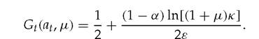
Differentiating the above expression yields our main theoretical predictions: The average growth rate decreases with exchange rate volatility, and this effect is stronger with a lower level of financial development as measured by μ.
In economies with high levels of financial development, exchange rate flexibility may enhance average growth by weeding
out the less innovative firms while promoting the more innovative. One should thus expect exchange rate flexibility to be more damaging to long-run growth when the degree of financial development is lower. This prediction turns out to be fully vindicated by the data. In particular, using a GMM panel data system estimator for 83 countries over a sequence of 5-year subperiods between 1961 and 2000, ABRR regress the growth rate of output per worker on exchange rate flexibility (computed from the same classification as in Rogoff et al.
(2003)) and its interaction with financial development. The results are summarized in Table 2.4. We see that the direct effect of exchange rate flexibility on growth is negative and significant, while the interaction term between financial development and exchange rate flexibility has a positve and significant coefficient. Thus, as predicted by the model above, the higher the degree of financial development, the less negative the effect of exchange rate flexibility on growth.This result may have interesting policy implications. For example, it may raise further questions for those European countries that are contemplating joining the EMU system. Given their level of financial development, should they tie their hands by adopting the Euro rather than maintaining a fully flexible exchange rate regime? The above result may also call for further organizational changes within the Euro zone, so that it would look more like one country with a flexible exchange rate vis-a-vis the rest of the world.
2.3.2 Productivity growth and countercyclical budgetary policy
Asecond avenue for policy analysis alsobasedon the basic insights of AABM, and currently explored by ABM, is to analyze budgetary policies over the business cycle and their effects on long-run growth. The above analysis showed that in countries with lower financial development, negative shocks or higher volatility have more damaging effects on mean R&D investment and growth. This, in turn, may suggest that countercyclical budgetary policies should be more growth-enhancing in countries with lower degrees of financial development.
For example, consider the following cross-country panel regression involving 19 OECD countries over the period 1961-2000, divided in 10-year subperiods. Budgetary policies are captured
Table 2.4 Regression of growth rate of output per worker on exchange rate flexibility
| Period: Unit of observation: Estimation technique: | 1961-2000 Non-overlapping 5-year averages System GMM | |||
| [1] | [2] | [3] | [4] | |
| Degree of Exchange | -0.1890* | —0.4405** | -1.1613** | -0.7847** |
| Flexibility (Rogoff et al. classification) | 0.1107 | 0.1728 | 0.3144 | 0.3392 |
| Financial Development | 0.8449** | 0.5420** | 0.7368** | 0.7108** |
| (private domestic credit/GDP, in logs) | 0.1292 | 0.2063 | 0.1903 | 0.2207 |
| Distance to Frontier | 0.0085 | -0.0424 | 0.7947** | 0.7108** |
| (log(Initial Output per worker US/Initial Output per worker)) | 0.0870 | 0.1136 | 0.1427 | 0.2207 |
| Flexibility*Financial | 0.1007** | 0.0976* | ||
| Development | 0.0504 | 0.0537 | ||
| Flexibility*Distance to | -0.5314** | -0.4844** | ||
| Frontier | 0.1018 | 0.1135 | ||
| Control variables Education | 0.8327** | 0.5420** | 0.8052** | 0.8617** |
| (secondary enrollment, in logs) | 0.1487 | 0.2063 | 0.1679 | 0.1778 |
| Trade Openness | 0.5471 ** | 0.6931 ** | 0.9036** | 1.0193** |
| (structure-adjusted trade volume/GDP, in logs) | 0.2162 | 0.2552 | 0.3177 | 0.3399 |
| Government Burden | -1.6837** | -0.4405** | -1.8885** | -17992** |
| (government consumption/GDP, in logs) | 0.2032 | 0.1728 | 0.2235 | 0.2766 |
| Lack of Price Stability | -4.0660** | -4.1598** | -3.5742** | -3.5272** |
| (inflation rate, in log [100+inf. rate]) | 0.4689 | 0.4792 | 0.4819 | 0.5535 |
| Intercept | 21.4569** | 22.7512** | 18.1347** | 18.5464** |
| 2.631951 | 2.8698 | 2.8700 | 3.5767 | |
Note: Dependent Variable: Growth Rate of Output per Worker (Standard errors are presented below the corresponding coefficient). **, * significant at the 5% and 10% respectively.
Table 2.5 Measure of countercyclicality of budgetary policies
| Period: 1961-2000, divided into four 10-year periods | |
| Distance to Frontier | -14.4913** 1.7072 |
| Education | 0.2222 0.1730 |
| Budgetary Activism | 1.7784** |
| (std. dev. of primary deficit over std. dev. of output gap1) | 0.7153 |
| Countercyclicality | 0.7336* |
| (correlation of primary budget deficit and output gap) | 0.4179 |
| Budgetary Activism*Financial Development | -0.0181** 0.0073 |
| Countercyclicality*Financial Development | -0.0106** 0.0044 |
| Intercept | 8.3357** 1.8130 |
Note: Dependent Variable: Growth Rate of Productivity (Standard errors are presented below the corresponding coefficient). **, * significant at the 5% and 10% respectively.
1 The output gap is measured as potential output minus actual output. Thus, a positive correlation implies countercyclical budgetary policy.
by two alternative measures. First, as a measure of budgetary activism, ABM use the ratio between the standard deviation of the primary deficit and the standard deviation of the output gap over a 10-year period. Second, ABM construct a measure of countercyclicality of budgetary policies by taking the average correlation between the primary deficit and the output gap over a 10-year period.4 One can regress productivity growth on these two variables and their interactions with financial development. The regression in Table 2.5 shows both, a positive and significant direct effect of budgetary activism on productivity growth, and positive and significant direct effect of countercyclicality of budgetary policy on productivity growth. More importantly, the interaction
4 Here, the output gap is measured as potential GDP minus actual GDP, implying that a positive correlation between the primary deficit and the output gap stands for countercyclical budgetary policy.
terms of both variables with financial development have negative and significant coefficients, which confirms the prediction that less financially developed economies should benefit more from countercyclical fiscal policies.
ABM intend to go further by performing two-stage regression procedures in which: (i) the first stage regresses government primary deficits for each country on the current output gap, the current departure from trend government expenditures, and debt repayments, under the assumption that governments pursue some kind of a tax smoothing objective (see Barro (1986) for theoretical foundations underlying such a first-stage specification); (ii) the second stage regresses average growth over a given period on financial development, the degree of countercyclicality of budgetary policy as it comes out of the first-stage regression for each country, and the interaction between financial development and the countercyclicality coefficient. This coefficient in turn replaces the previous two measures of activism and countercyclicality, now assuming that governments follow a prespecified objective. Preliminary results confirm the findings in Table 2.5, namely that countercyclical budgetary policies are more growth-enhancing when the level of financial development is lower. Interestingly, the European Union is less financially developed than the United States, and yet it advocates and also implements budgetary policies that are far less countercyclical than in the United States. Is that one among several potential explanations for the European stagnation vis-a-vis the United States?