Financial development and the effect of volatility on growth

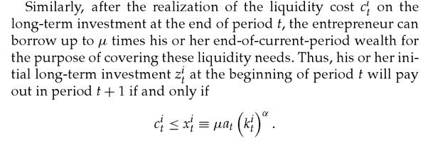
Let us augment the model of short- versus long-term investment developed in Section 1.3 of the previous chapter by introducing credit market imperfections. Thus, we assume that upon investing in short-run capital and in long-term investments, an entrepreneur born at date t can borrow only up to m times his or her initial wealth, so that he or she faces the investment constraint

where μ = 1 + m.

of credit constraints and as we might have expected, z_t falls with either a reduction in μ or an increase in φ.

Using the fact that

in equilibrium (in the absence of foreign lending or government bonds, and given that all entrepreneurs are ex ante identical with the same initial wealth so that there is no reason why one entre­preneur would end up lending to another entrepreneur in period t), we thus conclude that under sufficiently incomplete markets, the share ofR&D z_t becomes procyclical, and the share of capital investment k_t becomes countercyclical. Long-term investment z_t is less procyclical the less tight the credit constraints, less persistent the shocks, or longer the horizon of long-term investment.

The intuition for why long-term investment becomes more pro­cyclical when credit constraints are tighter, can be explained as follows: under tight credit constraints, a low realization of cur­rent productivity a_t means low level of profits a_t(k_t)^α at the end of the current period.

The above reasoning also implies that the tighter the credit con­straint, the more risky it is to invest in long-term investments in general, therefore the lower the mean long-term investment over time, and consequently the lower the average growth rate.

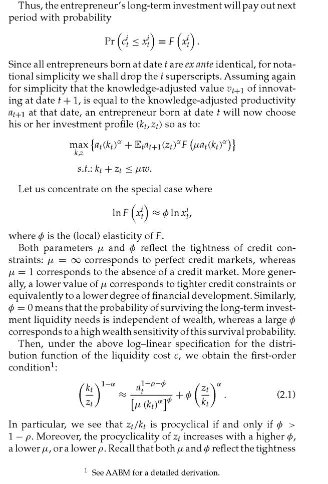
Example 1: The following two figures show how credit con­straints affect the level and procyclicality of long-term invest­ment. Here, we assume that the distribution of c is lognormal. We also assume that α = 1 /3, and we let μ vary between 1 (no credit) and 5.

Figure 2.1 depicts the equilibrium level of z_t, evaluated at the mean productivity level (a_t = 1). Figure 2.2 depicts the equilibrium

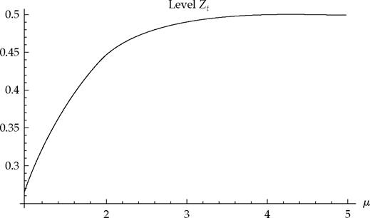
Fig. 2.1 The effect of incomplete markets on the level of long-term investment.

Source: AABM (2004), figure 2.

Fig. 2.2 The effect of incomplete markets on the cyclical elasticity of long-term investment.

Source: AABM (2004), figure 3.

cyclical elasticity of z_t (also evaluated at a_t = 1). In particular, we see that for μ sufficiently small, z_t is increasing in a_t ((dz_t/da_t) > 0): In other words, long-term investment becomes procyclical when μ is small and becomes countercyclical for μ sufficiently large.

We now turn our attention back to the effect of increased volat­ility on long-run average growth, and how it is affected by credit constraints.

of entrepreneurs will successfully meet the liquidity needs of long­term investment.

Now if we assume that knowledge grows at a rate proportional to the number of implemented (i.e. completed) innovations, then the growth rate of technology is now given by:

where z(a_t) is the (incomplete-markets) equilibrium level of long­term investment. Recall that in the absence of credit constraints (see Chapter 1) we simply had

since all innovations were always completed.

In fact, one can show that (z(a_t))^αδ(a_t) is always concave in a_t under the Cobb-Douglas long-term investment technology con­sidered in this chapter. Thus, the growth rate g_t is a concave function of a_t, and therefore mean growth will now fall in response to an increase in the variance of a_t (see Figure 2.3). Thus, in an eco­nomy with credit-constrained firms, an increase in volatility will result in lower mean growth.

Example 2: Assume linear production and long-term invest­ment technologies, namely:

Suppose also that the long-term growth-enhancing investment is indivisible, equal to some Zo ∈ (0, w), that the distribution for the liquidity shock”? is uniform over the interval [0,1], and that in the absence of volatility, firms could always pay? with their retained earnings from short-run production, more precisely:

where a is the average productivity shock.

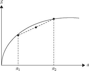
Fig. 2.3 Growth rate under Cobb-Douglas long-term investment technology.

Note: If we randomize between aj and a2, the average growth rate lies strictly below the curve.

We are interested in the effect of increased macroeconomic volat­ility (i.e. of increased variance of a, denoted by σ) on the expected growth rate

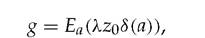
where

Since the liquidity shock is uniform, we have:

which is obviously concave in a. Figure 2.4 shows δ (a) as a function of a. In particular we see that randomizing between two values of a below and above the kink can only reduce the average δ so that volatility is unambiguously detrimental to average growth.

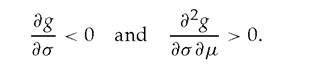
It then immediately follows that the expected growth rate g must decrease when the variance of a increases, and all the more when μ is lower. This result is quite intuitive: more volatility does not improve firms' ability to overcome the liquidity shock in a boom since firms already do it without volatility. However, it reduces the probability that they will overcome the liquidity shock in a slump, and to a larger extent when the firm faces tighter borrowing

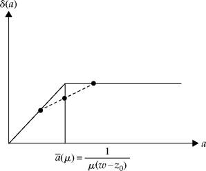
Fig. 2.4 Volatitlity is detrimental to average growth.

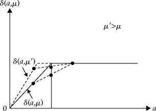
Fig. 2.5 Increased access to credit reduces the sensitivity of growth to productivity shocks.

constraints. We thus have:

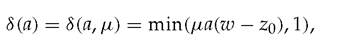
Moreover, the ex post growth rate,

is increasing and concave in a, but becomes constant and equal to λzo when μ is sufficiently large.

Thus, increased access to credit (a higher μ) reduces the sens­itivity of growth to productivity shocks and also the extent to which volatility is detrimental to growth (since growth becomes less concave in a).

2.1.1 Main theoretical predictions

To complete this section we list our main predictions as they emerge from our above discussion:

1. Long-term investment tends to be countercyclical in the absence of credit constraints, but becomes increasingly pro­cyclical as credit constraints tighten.

2. When firms face tighter credit constraints, the effect of volat­ility on expected average growth tends to become more negative (or less positive).

3. When firms face tighter constraints, growth becomes more sensitive to exogenous shocks.

2.2