Empirics of poverty traps

Casual observation of the cross-country income panel tends to suggest mechanisms which reinforce wealth or poverty. In Section 4.1 we review the main facts. Section 4.2 considers tests for the empirical relevance of poverty trap models.

4.1. Bimodality and convergence clubs

A picture of the evolving cross-country income distribution is presented in Figure 14. For both the top and bottom histograms the y-axis measures frequency. For the top pair (1960 and 1995) the x-axis is GDP per capita in 1996 PPP adjusted dollars. This is the

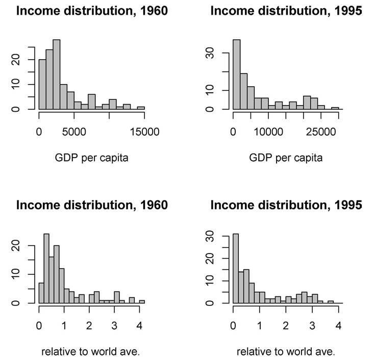
Figure 14.

standard histogram of the cross-country income distribution. For the bottom pair the x-axis represents income as a fraction of the world average for that year.

The single most striking feature of the absolute income histograms for 1960 and 1995 is that over this period a substantial fraction of poor countries have grown very little or not at all. At the same time, a number of middle income countries have grown rapidly, in some cases fast enough to close in on the rich. Together, these forces have caused the distribution to become somewhat thinner in the middle, with probability mass collecting at the two extremes. Such an outcome is consistent with mechanisms that accentuate differences in initial conditions, and reinforce wealth or poverty [Azariadis and Drazen (1990), Quah (1993, 1996), Durlauf and Johnson (1995), Bianchi (1997), Pritchett (1997), Desdoigts (1999), Easterly and Levine (2000)].

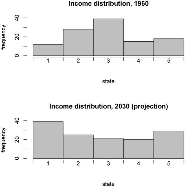
Figure 15.

nonparametric, the projections do not contain any of the restrictions implied by growth theory.

Quah (1996) addressed the first of these problems by estimating a continuous state version. In the language of this survey, he estimates a stochastic kernel Γ, of which P is a discretized representation. The estimation is nonparametric, using a Parzen-window type density smoothing technique. The kernel is suggestive of considerable persistence.

Azariadis and Stachurski (2004) make some effort to address both the discretization problem and the lack of economic theory simultaneously, by estimating Γ parametri­cally, using a theoretical growth model. In essence, they estimate Equation (9), where k → A(k) is represented by a three-parameter logistic function. The logistic function nests a range of growth models, from the convex model in Figure 2 to the nonconvex models in Figure 7, panels (a), (b) and (d). Once the law of motion (9) is estimated, the stochastic kernel Γ is calculated via Equation (10), and the projection of distributions is computed by iterating (4).

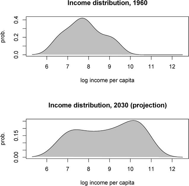
Figure 16.

The resulting 2030 prediction is shown in Figure 16, with the 1960 distribution drawn above for comparison. The x-axis is log of real GDP per capita in 1996 US dollars. The 1960 density is just a smoothed density estimate using Gaussian kernels, with data from the Penn World Tables. The same data was used to estimate the parameters in the law of motion (9). AsinFigure 15, a unimodal distribution gives way to a bimodal distribution.

These findings do lend some support to Quah’s convergence club hypothesis. Much work remains to be done. For example, in all of the methodologies discussed above, nonstationary data is being fitted to a stationary Markov chain. This is clearly a source of bias. Furthermore, all of these models are too small, in the sense that the state space used in the predictions are only one-dimensional.^[236]

4.2. Testing for existence

Poverty trap models tend to be lacking in testable quantitative implications. Where there are multiple equilibria and sensitive dependence to initial conditions, outcomes are much harder to pin down than when the map from parameters to outcomes is ro­bust and unique. This has led many economists to question the empirical significance of poverty trap models.⁴⁸ In this section, we ask whether or not there is any evidence that poverty traps exist.

In answering this question, one must be very careful to avoid the following circular logic: First, persistent poverty is observed. Poverty traps are then offered as the expla­nation. But how do we know there are poverty traps? Because (can’t you see?) poverty persists.⁴⁹ This simple point needs to be kept in mind when interpreting the data with a view to assessing the empirical relevance of the models in this survey. Persistentpoverty, emergent bimodality and the dispersion of cross-country income are the phenomena we seek to explain. They cannot themselves be used as proof that poverty traps explain the data.

Also, a generalized convex neoclassical model can certainly be the source of bimodal­ity and dispersion if we accept that the large differences in total factor productivity residuals across countries are due to some exogenous force, the precise nature of which is still waiting to be explained. In this competing explanation, the map from funda­mentals to outcomes is unique, and shocks or historical accidents which perturb the endogenous variables can safely be ignored.

The central question, then, is whether or not the poverty trap explanation of cross­country income differentials survives if we control for the exogenous forces which determine long run economic performance. In other words, do self-reinforcing and path dependent mechanisms imply that economies populated by fundamentally simi­lar people in fundamentally similar environments can support very different long run outcomes? What empirical support is there for such a hypothesis?

One particularly interesting study which addresses this question is that of Bloom, Canning and Sevilla (2003). Their test is worth discussing in some detail. To begin, consider again the two multiple equilibria models shown in Figure 8 (Section 3.3), along with their ergodic distributions. As can be seen in the left hand panels, when the shock is suppressed both Country A and Country B have two locally stable equilibria for capital per worker - and therefore two locally stable equilibria for income. Call these two states yj^t and yf the first of which is interpreted as the poverty trap.

yield a process which is not generally Markovian. Moreover, there are interactions between countries that affect economic performance, and these interactions are important. A first-best approach would be to treat the world economy as an N ? M-dimensional Markov process, where N is the number of countries, and M is the number of endogenous variables in each country. One would then estimate the stochastic kernel Γ for this process, a map from >ⁿ?^m ? >ⁿ?^m → [0, ∞). Implications for the cross-country income distribution could be calculated by computing marginals.

⁴⁸ See Matsuyama (1997) for more discussion of this point.

⁴⁹ Recall Karl Popper’s famous tale about Neptune and the sea.

In general, y{ and y⅛ will depend on the vector of exogenous fundamentals, which determine the exact functional relationships in the model, and hence become parame­ters in the law of motion.

Here p(x) is the probability that the country in question is in the basin of attraction for the lower equilibrium y₁* (x) at time t. This probability is determined by the time t mar­ginal distribution of income. The shock u_i represents deviation from the deterministic attractor at time t.

Figure 8 helps to illustrate how y₁* and y⅛ might depend on the exogenous variables. Imagine that Countries A and B have characteristics õ_ä and x_B respectively. These different characteristics account for the different shapes of the laws of motion shown in the left-hand side of the figure. As drawn, y⅛ (õ_ä), the high level attractor for Country A, is less than y^(x_B), the high level attractor for Country B, while y₁* (õ_ä) and y₁* (x_B) are roughly equal.

In addition, we can see how the probability p(x) of being in the poverty trap basin depends on these characteristics. For time t sufficiently large, ergodicity means that the time t marginal distribution - which determines this probability - can be identified with the ergodic distribution. The ergodic distribution in turn depends on the underlying structure, which depends on x. This is illustrated by the different sizes of the distribution modes for Countries A and B in Figure 8. For Country A the left hand mode is relatively large, and hence so is p(x).

Using a maximum likelihood ratio test, the specification (R2) is evaluated against a single regime alternative which can be thought of for the moment as being generated by a convex Solow model. The great benefit of the specifications (R1) and (R2) - as emphasized by the authors - is that long run output depends only on exogenous factors.

In conducting the test of (R1) against (R2), it is important not to include as exogenous characteristics any variable which is in fact endogenously determined. For to do so might result in conditioning on the outcomes of the underlying process which generates multiple equilibria. In the words of the authors, “Including such variables may give the impression of a unique equilibrium relationship [for the economic system] when in reality they are a function of the equilibrium being observed. Fundamental forces must be characteristics that determine a country’s economic performance but are not determined by it.”

In the estimation of Bloom, Canning and Sevilla, only geographic features are in­cluded in the set of exogenous variables. These include data on distance from equator, rainfall, temperature, and percentage of land area more than 100 km from the sea. For this set of variables, the likelihood ratio test rejects the single regime model (R1) in favor of the multiple equilibria model (R2). They find evidence for a high level equilib­rium which does not vary with x, and a low level equilibrium which does. In particular, yl (x) tends to be smaller for hot, dry, land-locked countries (and larger for those with more favorable geographical features). In addition, p(x) is larger for countries with un­favorable geographical features. In other words, the mode of the ergodic distribution around (x) is relatively large. For these economies escape from the poverty trap is more difficult.

Overall, the results of the study support the poverty trap hypothesis. They also serve to illustrate the importance of distinguishing between variables which are exogenous and those which have feedback from the system. If one conditions on “explanatory” variables which deviate significantly from fundamental forces, the likelihood of ob­serving multiple equilibria in the map from those variables to outcomes will be lower. For example, one theme of this survey is that institutions can be an important source of multiplicity, either directly or indirectly through their interactions with the mar­ket. If institutions are endogenous, and if traps in institutions drive the disparities in cross-country incomes, then conditioning on institutions may give spurious convergence results entirely disconnected from long run outcomes generated by the system.

4.3. Model calibration

One of the advantages of the methodology proposed by Bloom, Canning and Sevilla is that estimation and testing can proceed without fully specifying the underlying model. The exacting task of determining the relevant set of endogenous variables and the laws by which they interact is thereby circumvented. But there are two sides to this coin. While the results of the test suggest that poverty traps matter, they give no indication as to their source, or to the appropriate framework for formulating them as models.

Graham and Temple (2004) take the opposite approach. They give the results of a numerical experiment starting from a specific poverty trap model, somewhat akin to the inertial self-reinforcement model of Section 3.4. The question they ask is whether or not the model in question has the potential to explain observed cross-country variation in per capita income for a reasonable set of parameters. We briefly outline their main findings, as well as their technique for calibration, which is of independent interest.

As in Section 3.4, there is both a traditional agricultural sector and a modern sector with increasing social returns due to technical externalities. The agricultural sector has a decreasing returns technology

Ya = A_aL^γ_a, γ ∈ (0, 1),

(11)

where Y_a is output, A_a is a productivity parameter and L_a is labor employed in the agricultural sector. The j th firm in the modern sector has technology

Using this strategy and a more elaborate model (including both capital and land), Gra­ham and Temple’s main findings are as follows. First, for reasonable parameter values some 1 /4 of the 127 countries in their 1988 data set are in the poverty trap α⅛. Second, after calculating the variance of log income across countries when all are in their high output equilibrium and comparing it to the actual variance of log income, they find that the poverty trap model can account for some 2/5 to one half of all observed variation in incomes.

Overall, their study suggests that the model can explain some properties of the data, such as the difference between poor, agrarian economies and low to middle income countries. On the other hand, it cannot account for the huge differences between the very poorest and the rich industrialized countries. In the model, the largest ratios of

51

See, for example, Caballero and Lyons (2002).

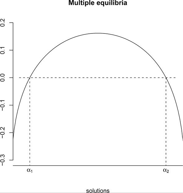
Figure 17.

low to high equilibrium production are in the region of two to three. As we saw in Section 2.1, however, actual per capita output ratios between rich and poor countries are much larger.

4.4. Microeconomicdata

There has also been research in recent years on poverty traps that occur at the individual or group level. For example, Jalan and Ravallion (2002) fit a microeconomic model of consumption growth with localized spillovers to farm-household panel data from rural China. Their results are consistent with empirical significance of geographical poverty traps. Other authors have studied particular trap mechanisms. For example, Bandiera and Rasul (2003) and Conley and Udry (2003) consider the effects of positive network externalities on technology adoption in Mozambique and Ghana respectively. Barrett, Bezuneh and Aboud (2001) consider the dynamic impact of credit constraints on the poor in Cote d’Ivoire and Kenya. Morduch (1990) studies the effect of risk on income in India, as does Dercon (1998) for Tanzania.

5.