3. Models and definitions

We begin our attempt to answer the question posed at the end of the last section with a review of the convex neoclassical growth model. It is appropriate to start with this model because it is the benchmark from which various deviations will be considered.

3.1. Neoclassical growth with diminishing returns

The convex neoclassical model [Solow (1956)] begins with an aggregate production function of the form

¹² The figures are from Maddison (1995). His units are 1990 international dollars.

Because of diminishing returns, capital poor countries will extract greater marginal returns from each unit of capital stock invested than will countries with plenty of capital. The result is convergence to a long-run outcome which depends only on fundamental primitives (as opposed to beliefs, say, or historical conditions).

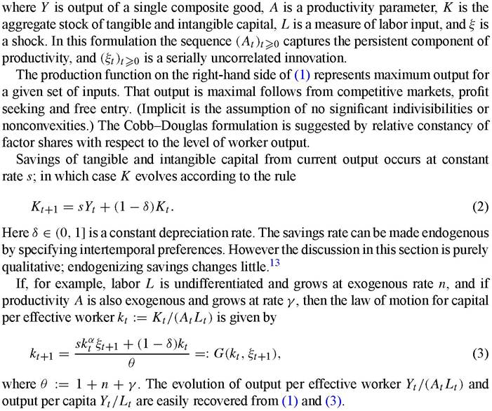
Figure 2 shows the usual deterministic global convergence result for this model when the shock ξ is suppressed. The steady state level of capital per effective worker is k_b. Figure 3 illustrates stochastic convergence with three simulated series from the law of motion (3), one with low initial income, one with medium initial income and one with high initial income. Part (a) of the figure gives the logarithm of output per effective worker, while (b) is the logarithm of output per worker.

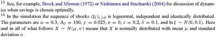
15

See Appendix A for details.

Figure 3.

All Markov processes have the property that the sequences of marginal distributions they generate satisfies a recursion in the form of (4) for some stochastic kernel Γ.17 Although the state variables usually do not themselves become stationary (due to the ongoing presence of noise), the sequence of probabilities (ψ_t)_t≥0 may. In particular, the following behavior is sometimes observed: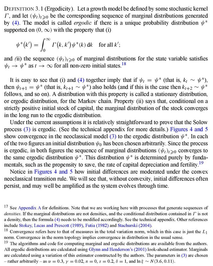

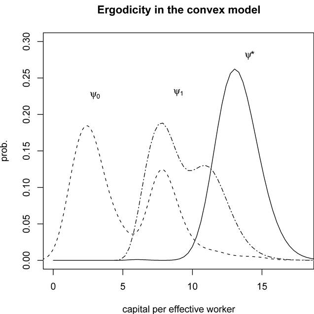
Figure 4.

3.2. Convex neoclassical growth and the data

The convex neoclassical growth model described in the previous section predicts that per capita incomes will differ across countries with different rates of physical and human capital formation or fertility. Can the model provide a reasonable explanation then for the fact that per capita income in the US is more than 70 times that in Tanzania or Malawi?

The short answer to this question is no. First, rates at which people accumulate re­producible factors of production or have children (fertility rates) are endogenous - in fact they are choice variables. To the extent that factor accumulation and fertility are important, we need to know why some individuals and societies make choices that lead them into poverty. For poverty is suffering, and, all things being equal, few people will choose it.

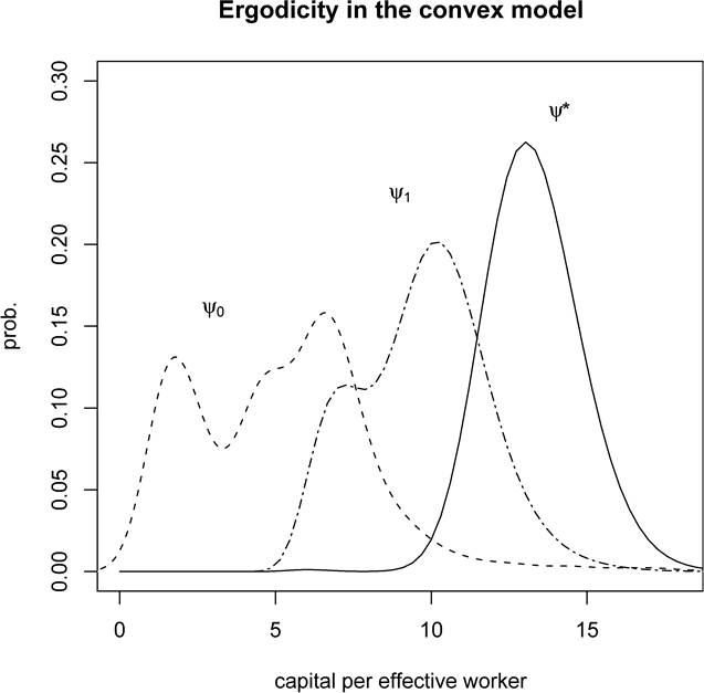
Figure 5.

This same observation leads us to suspect that the choices facing individuals in rich countries and those facing individuals in poor countries are very different. In poor coun­tries, the choices that collectively would drive modern growth - innovation, investment in human and physical capital, etc. - must be perceived by individuals as worse than those which collectively lead to the status quo.^[219]

A second problem for the convex neoclassical growth model as an explanation of level differences is that even when we regard accumulation and fertility rates as ex­ogenous, they must still account for all variation in income per capita across countries. However, as many economists have pointed out, the differences in savings and fertility rates are not large enough to explain real income per capita ratios in the neighborhood of 70 or 100. A model ascribing output variation to these few attributes alone is insuf­ficient. A cotton farmer in the US does not produce more cotton than a cotton farmer in Mali simply because he has saved more cotton seed. The production techniques used in these two countries are utterly different, from land clearing to furrowing to plant­ing to irrigation and to harvest. A model which does not address the vast differences in production technology across countries cannot explain the observed differences in output.

Let us very briefly review the quantitative version of this argument.²¹ To begin, recall the aggregate production function (1), which is repeated here for convenience:

All of the components are more or less observable besides A_t and the shock.²² Hall and Jones (1999) conducted a simple growth accounting study by collecting data on the observable components for the year 1988. They calculate that the geometric average of output per worker for the 5 richest countries in their sample was 31.7 times that of the 5 poorest countries.

This is not a promising start for the neoclassical model as a theory of level differences. Essentially, it says that there is no single map from total inputs to aggregate output that holds for every country. Why might this be the case? We know that the aggregate pro­duction function is based on a great deal of theory. Output is maximal for a given set of inputs because of perfect competition among firms. Free entry, convex technology relative to market size, price taking and profit maximization mean that the best tech­nologies are used - and used efficiently. Clearly some aspect of this theory must deviate significantly from reality.

Now consider how this translates into predictions about level differences in income per capita. When the shock is suppressed (ξ_t = 1 for all t), output per capita converges to the balanced path

²¹ The review is brief because there are many good sources. See, for example, Lucas (1990), King and Rebelo (1993), Prescott (1998), Hall and Jones (1999) or Easterly and Levine (2000).

²² The parameter α is the share of capital in the national accounts. Human capital can be estimated by collect­ing data on total labor input, schooling, and returns to each year of schooling as a measure of its productivity.

²³ The domestic production shocks (ξ_t)_t >0 are not the source of the variation. This is because they are very small relative to the differences in incomes across countries, and, by definition, not persistent. (Recall that in our model they are innovations to the permanent component (At)_t>0∙)

²⁴ When considering income levels it is necessary to assume that countries are in the neighborhood of the balanced path, for this is where the model predicts they will be.

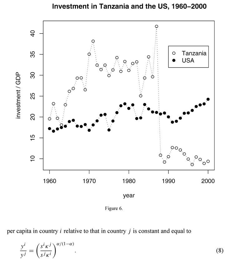
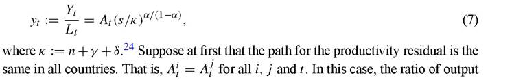
The problem for the neoclassical model is that the term inside the brackets is usually not very large. For example, if we compare the US and Tanzania, say, and if we identify capital with physical capital, then average investment as a fraction of GDP between 1960 and 2000 was about 0.2 in the US and 0.24 in Tanzania. (Although the rate in Tanzania varied a great deal around this average. See Figure 6.) The average population growth rates over this period were about 0.01 and 0.03 respectively. Since A^l_t = A^j for all t we have γ^l = γ^j. Suppose that this rate is 0.02, say, and that δ^l = δ^j = 0.05. This gives s^lκ^j/(s^jκ^l) ~ 1. Since payments to factors of production suggest that α∕(1 — α) is neither very large nor very small, output per worker in the two countries is predicted to be roughly equal.

This is only an elementary calculation. The computation of investment rates in Tan­zania is not very reliable. There are issues in terms of the relative ratios of consumption and investment good prices in the two countries which may distort the data. Further, we have not included intangible capital - most notably human capital. The rate of investment in human capital and training in the US is larger than it is in Tanzania. Nevertheless, it is difficult to get the term in (8) to contribute a factor of much more than 4 or 5 - certainly not 70.^[220]

However the calculations are performed, it turns out that to explain the ratio of in­comes in countries such as Tanzania and the US, productivity residuals must absorb most of the variation. In other words, the convex neoclassical growth model cannot be reconciled with the cross-country income data unless we leave most of the variation in income to an unexplained residual term about which we have no quantitative theory.

Different authors have made this same point in different ways. Lucas (1990) notes that if factor input differences are large enough to explain cross-country variations in income, the returns to investment in physical and human capital in poor countries im­plied by the model will be huge compared to those found in the rich. They are not. Also, productivity residuals are growing quickly in countries like the US.^[221] On the other hand, in countries like Tanzania, growth in the productivity residual has been very small.^[222] Yet the convex neoclassical model provides no theory on why these different rates of growth in productivity should hold.

On balance, the importance of productivity residuals suggests that the poor countries are not rich because for one reason or another they have failed or not been able to adopt modern techniques of production. In fact production technology in the poorest countries is barely changing. In West Africa, for example, almost 100% of the increase in per capita food output since 1960 has come from expansion of harvest area [Baker (2004)]. On the other hand, the rich countries are becoming ever richer because of continued innovation.

Of course this only pushes the question one step back. Technological change is only a proximate cause of diverging incomes. What economists need to explain is why pro­duction technology has improved so quickly in the US or Japan, say, and comparatively little in countries such as Tanzania, Mali and Senegal.

We end this section with some caveats. First, the failure of the simple convex neo­classical model does not imply the existence of poverty traps. For example, we may discover successful theories that predict very low levels of the residual based on ex­ogenous features which tend to characterize poor countries. (Although it may turn out that, depending on what one is prepared to call exogenous, the map from fundamentals to outcomes is not uniquely defined. In other words, there are multiple equilibria. In Section 4.2 some evidence is presented on this point.)

Further, none of the discussion in this section seeks to deny that factor accumulation matters. Low rates of factor accumulation are certainly correlated with poor perfor­mance, and we do not wish to enter the “factor accumulation versus technology” debate - partly because this is viewed as a contest between neoclassical and “endogenous” growth models, which is tangential to our interests, and partly because technology and factor accumulation are clearly interrelated: technology drives capital formation and investment boosts productivity.^[223]

Finally, it should be emphasized that our ability to reject the elementary convex neo­classical growth model as a theory of level differences between rich and poor countries is precisely because of its firm foundations in theory and excellent quantitative proper­ties. All of the poverty trap models we present in this survey provide far less in terms of quantitative, testable restrictions that can be confronted with the data. The power of a model depends on its falsifiability, not its potential to account for every data set.

3.3. Poverty traps: historical self-reinforcement

How then are we to explain the great variation in cross-country incomes such as shown in Figure 1? In the introduction we discussed some deviations from the neoclassical benchmark which can potentially account for this variation by endogenously reinforcing small initial differences. Before going into the specifics of different feedback mecha­nisms, this section formulates the first of two abstract poverty trap models. For both models a detailed investigation of microfoundations is omitted. Instead, our purpose is to establish a framework for the questions poverty traps raise about dynamics, and for their observable implications in terms of the cross-country income data.

The first model - a variation on the convex neoclassical growth model discussed in Section 3.1 - is loosely based on Romer (1986) and Azariadis and Drazen (1990). It exemplifies what Mookherjee and Ray (2001) have called historical self-reinforcement, a process whereby initial conditions of the endogenous variables can shape long run outcomes. Leaving aside all serious complications for the moment, let us fix at s > 0 the savings rate, and at zero the rates of exogenous technological progress γ and population growth n. Let all labor be undifferentiated and normalize its total mass to 1, so that k represents both aggregate capital and capital per worker. Suppose that the productivity parameter A can vary with the stock of capital. In other words, A is a function of k, and aggregate returns k_t → A(k_t)k^lj^t are potentially increasing.^[224]

The law of motion for the economy is then

Depending on the specification of the relationship between k and productivity, many dynamic paths are possible. Some of them will lead to poverty traps. Figure 7 gives examples of potential dynamic structures. For now the shock ξ is suppressed. The x -axis is current capital k_t and the y-axis is k_t+1. In each case the plotted curve is just the right­hand side of (9), all with different maps k → A(k).

In part (a) of the figure the main feature is non-ergodic dynamics: long run outcomes depend on the initial condition. Specifically, there are two local attractors, the basins of attraction for which are delineated by the unstable fixed point k_b. Part (b) is also non- ergodic. It shows the same low level attractor, but now no high level attractor exists. Beginning at a state above k_b leads to unbounded growth. In part (c) the low level attractor is at zero.

The figure in part (d) looks like an anomaly. Since the dynamics are formally ergodic, many researchers will not view this structure as a “poverty trap” model. Below we argue that this reading is too hasty: the model in (d) can certainly generate the kind of persistent-poverty aggregate income data we are hoping to explain.

In order to gain a more sophisticated understanding, let us now look at the stochastic dynamics of the capital stock. Deterministic dynamics are of course a special case of stochastic dynamics (with zero-variance shocks) but as in the case of the neoclassical model above, let us suppose that (ξ_t)_t ≥₀ is independently and identically lognormally distributed, with lnξ ~ N(μ, σ) and σ > 0. It then follows that the sequence of marginal distributions (ψ_t)_t≥₀ for the capital stock sequence (k_t)_t≥₀ again obeys the recursion (4) where the stochastic kernel Γ is now

with φ the lognormal density on (0, ∞) and zero elsewhere. All of the intuition for the recursion (4) and the construction of the stochastic kernel (10) is exactly the same as the neoclassical case.

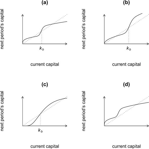
Figure 7.

³⁰ In fact we require also that k → A(k) is a Borel measurable function. But this condition is very weak indeed. For example, k → A(k) need be neither monotone nor continuous.

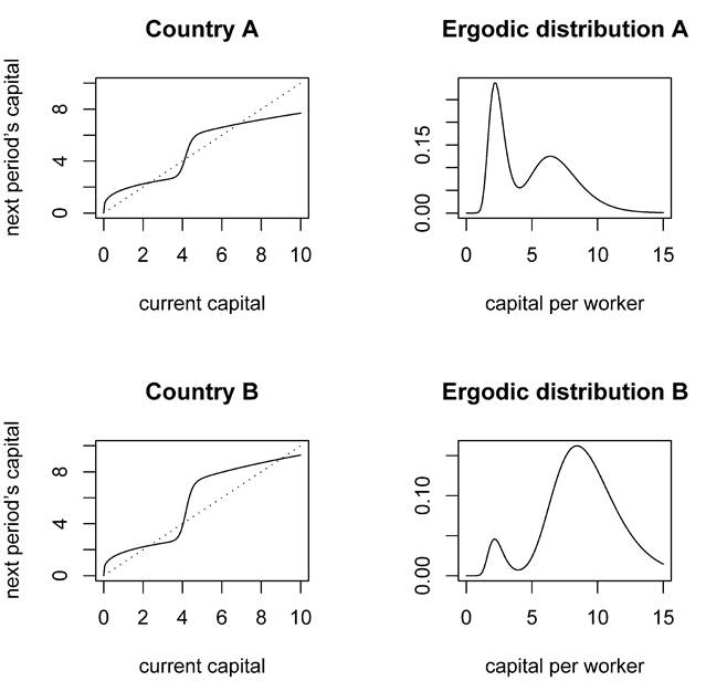
Figure 8.

Ergodicity here refers to Definition 3.1, which, incidentally, is the standard defini­tion used in growth theory and macroeconomics [see, for example, Brock and Mirman (1972); or Stokey, Lucas and Prescott (1989)]. In other words, there is a unique ergodic distribution ψ*, and the sequence of marginal distributions (ψ_t)_t≥₀ converges to ψ* asymptotically, independent of the initial condition (assuming of course that k₀ > 0). A proof of this result is given in Appendix A.

So why has a non-ergodic model become ergodic with the introduction of noise? The intuition is completely straightforward: Under our assumption of unbounded shocks there is always the potential - however small - to escape any basin of attraction. So in the long run initial conditions do not matter. (What does matter is how long this long run is, a point we return to below.)

Figure 8 gives the ergodic distributions corresponding to two poverty trap models.^[225] Both have the same structural dynamics as the model in part (a) of Figure 7. The left hand panels show this structure with the shock suppressed. The right hand panels show corresponding ergodic distributions under the independent lognormal shock process. Both ergodic distributions are bimodal, with modes concentrated around the determin­istic local attractors.

31

Comparing the two left hand panels, notice that although qualitatively similar, the laws of motion for Country A and Country B have different degrees of increasing re­turns. For Country B, the jump occurring around k = 4 is larger. As a result, the state is less likely to return to the neighborhood of the lower attractor once it makes the transition out of the poverty trap. Therefore the mode of the ergodic distribution corre­sponding to the higher attractor is large relative to that of Country A. Economies driven by law of motion B spend more time being rich.

Convergence to the ergodic distribution in a nonconvex growth model is illustrated in Figure 9. The underlying model is (a) of Figure 7.32 As before, the ergodic distribution is bimodal. In this simulation, the initial distribution was chosen arbitrarily. Note how initial differences tend to be magnified over the medium term despite ergodicity. The initially rich diverge to the higher mode, creating the kind of “convergence club” effect already seen in ψ₁₅, the period 15 marginal distribution.³³

It is clear, therefore, that ergodicity is not the whole story. If the support of the shock ξ is bounded then ergodicity may not hold. Moreover, even with ergodicity, historical conditions may be arbitrarily persistent. Just how long they persist depends mainly on (i) the size of the basins of attraction and (ii) the statistical properties of the shock. On the other hand, the non-zero degree of mixing across the state space that drives ergodicity is usually more realistic than deterministic models where poverty traps are absolute and can never be overcome. Indeed, we will see that ergodicity is very useful for framing empirical questions in Section 4.2.

Figures 10 and 11 illustrate how historical conditions persist for individual time series generated by a model in the form of (a) of Figure 7, regardless of ergodicity. In both figures, the x-axis is time and the y-axis is (the log of) capital stock per worker. The dashed line through the middle of the figure corresponds to (the log of) k_b, the point dividing the two basins of attraction in (a) of Figure 7. Both figures show the simulated time series of four economies. In each figure, all four economies are identical, apart from their initial conditions. One economy is started in the basin of attraction for the higher attractor, and three are started in that of the lower attractor.³⁴

In the figures, the economies spend most of the time clustered in the neighborhoods of the two deterministic attractors. Economies starting in the portion of the state space

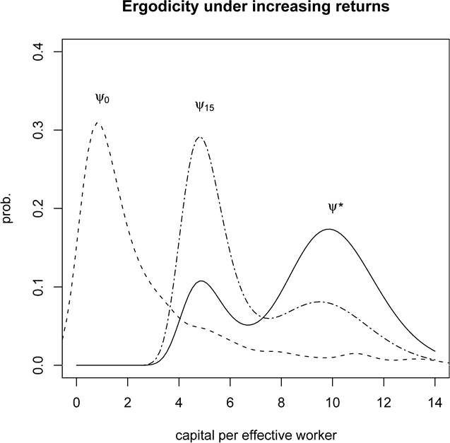
Figure 9.

(the y-axis) above the threshold are attracted on average to the high level attractor, while those starting below are attracted on average to the low level attractor. For these parameters, historical conditions are important in determining outcomes over the kinds of time scales economists are interested in, even though there are no multiple equilibria, and in the limit outcomes depend only on fundamentals.

In Figure 10, all three initially poor economies eventually make the transition out of the poverty trap, and converge to the neighborhood of the high attractor. Such transitions might be referred to as “growth miracles”. In these series there are no “growth disasters” (transitions from high to low). The relative likelihood of growth miracles and growth disasters obviously depends on the structure of the model - in particular, on the relative size of the basins of attraction.

In Figure 10 the shock is distributed according to lnξ ~ N(0, 0.1), while in Fig­ure 11 the variance is smaller: lnξ ~ N(0, 0.05). Notice that in Figure 11 no growth

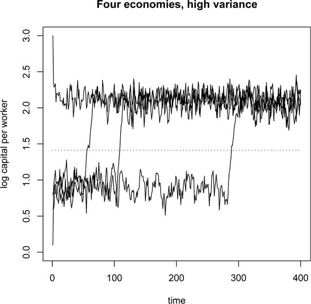
Figure 10.

miracles occur over this time period. The intuition is clear: With less noise, the proba­bility of a large positive shock - large enough to move into the basin of attraction for the high attractor - is reduced, and with it the probability of escaping from the poverty trap.

We now return to the model in part (d) of Figure 7, which is nonconvex, but at the same time is ergodic even in the deterministic case. This kind of structure is usually not regarded as a poverty trap model. In fact, since (d) is just a small perturbation of model (a), the existence of poverty traps is often thought to be very sensitive to parame­ters - a small change can cause a bifurcation of the dynamics whereby the poverty trap disappears. But, in fact, the phenomenon of persistence is more subtle. In terms of their medium run implications for cross-country income patterns, the two models (a) and (d) are very similar.

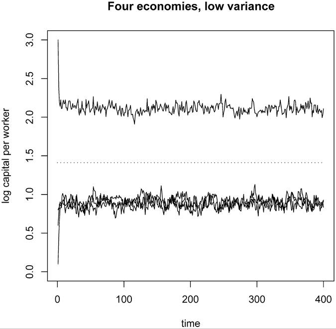
Figure 11.

To illustrate this, Figure 12 shows an arbitrary initial distribution and the resulting time 5 distribution for k under the law of motion given in (d) of Figure 7.^[226] As in all cases we have considered, the stochastic model is ergodic. Now the ergodic distribution (not shown) is unimodal, clustered around the single high level attractor of the deter­ministic model. Thus the long run dynamics are different to those in Figure 9. However, during the transition, statistical behavior is qualitatively the same as that for models that do have low level attractors (such as (a) of Figure 7). In ψ₅ we observe amplification of initial differences, and the formation of a bimodal distribution with two “convergence clubs”.

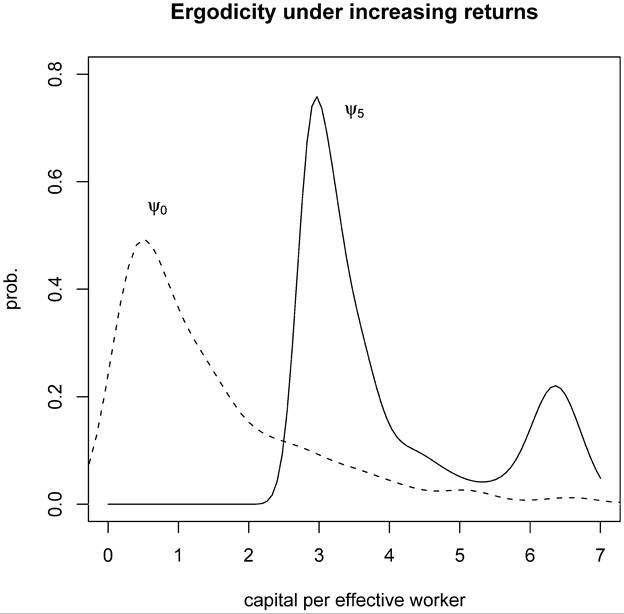
Figure 12.

How long is the medium run, when the transition is in progress and the distribution is bimodal? In fact one can make this transition arbitrarily long without changing the basic qualitative features of (d), such as the non-existence of a low level attractor. Its length depends on the degree of nonconvexity and the variance of the productivity shocks (ξ_t)_t^₀. Higher variance in the shocks will tend to speed up the transition.

Incidentally, the last two examples have illustrated an important general principle: In economies with nonconvexities, the dynamics of key variables such as income can be highly sensitive to the statistical properties of the exogenous shocks which perturb activity in each period.^[227] This phenomenon is consistent with the cross-country income panel. Indeed, several studies have emphasized the major role that shocks play in de­termining the time path of economic development [cf., e.g., Easterly et al. (1993), Den Haan (1995), Acemoglu and Zilibotti (1997), Easterly and Levine (2000)].^[228]

At the risk of some redundancy, let us end our discussion of the increasing returns model (9) by reiterating that persistence of historical conditions and formal ergodicity may easily coincide. (Recall that the time series in Figure 11 are generated by an ergodic model, and that (d) of Figure 7 is ergodic even in the deterministic case.) As a result, identifying history dependence with a lack of ergodicity can be problematic. In this survey we use a more general definition:

Definition 3.2 (Poverty trap). A poverty trap is any self-reinforcing mechanism which causes poverty to persist.

When considering a given quantitative model and its dynamic implications, the im­portant question to address is, how persistent are the self-reinforcing mechanisms which serve to lock in poverty over the time scales that matter when welfare is computed?^[229]

A final point regarding this definition is that the mechanisms which reinforce poverty may occur at any scale of social and spatial aggregation, from individuals to families, communities, regions, and countries. Traps can arise not just across geographical lo­cation such as national boundaries, but also within dispersed collections of individuals affiliated by ethnicity, religious beliefs or clan. Group outcomes are then summed up progressively from the level of the individual.^[230]

3.4. Poverty traps: inertial self-reinforcement

Next we turn to our second “canonical” poverty trap model, which again is presented in a very simplistic form. (For microfoundations see Sections 5-8.) The model is static rather than dynamic, and exhibits what Mookherjee and Ray (2001) have described as inertial self-reinforcement.^[231] Multiple equilibria exist, and selection of a particular equilibrium can be determined purely by beliefs or subjective expectations.

in the economy a unit mass of agents choose to work either in a traditional, rural sector or a modern sector. Labor is the only input to production, and each agent supplies one unit in every period. All markets are competitive. in the traditional sector returns to scale are constant, and output per worker is normalized to zero. The modern sector, however, is knowledge-intensive, and aggregate output exhibits increasing returns due perhaps to spillovers from agglomeration, or from matching and network effects.

Traditional and modern sector returns

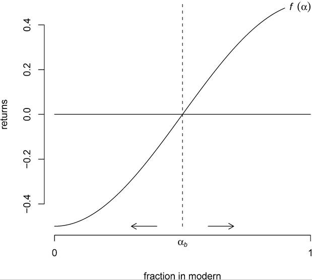
Figure 13.

Let the fraction of agents working in the modern sector be denoted by α. The map α → f(α) gives output per worker in the modern sector as a function of the frac­tion employed there. Payoffs are just wages, which equal output per worker (marginal product). Agents maximize individual payoffs taking the share α as exogenously given.

We are particularly interested in the case of strategic complementarities. Here, entry into the modern sector exhibits complementarities if the payoff to entering the modern sector increases with the number of other agents already there; in other words, if f is increasing. We assume that f' > 0, and also that returns in the modern sector dominate those in the traditional sector only when the number of agents in the modern sector rises above some threshold. That is, f(0)< 0 < /(1). This situation is shown in Figure 13. At the point α_b returns in the two sectors are equal.

Equilibrium distributions of agents are values of α such that f(α) = 0, as well as “all workers are in the traditional sector”, or “all workers are in the modern sector” (ignoring adjustments on null sets). The last two of these are clearly Pareto-ranked: The equilibrium α = 0 has the interpretation of a poverty trap.

Immediately the following objection arises. Although the lower equilibrium is to be called a poverty trap, is there really a self-reinforcing mechanism here which causes poverty to persist? After all, it seems that as soon as agents coordinate on the good equilibrium “poverty” will disappear. And there are plenty of occasions where societies acting collectively have put in place the institutions and preconditions for successful coordination when it is profitable to do so.

Although the last statement is true, it seems that history still has a role to play in equilibrium selection. This argument has been discussed at some length in the liter­ature, usually beginning with myopic Marshallian dynamics, under which factors of production move over time towards activities where returns are higher. In the case of our model, these dynamics are given by the arrows in Figure 13. If (α₀)_t≥₀ is the se­quence of modern sector shares, and if initially α₀ < a_b, then α_t → 0. Conversely, if α₀ > a_b, then α_t → 1.

But, as many authors have noted, this analysis only pushes the question one step back. Why should the sectoral shares only evolve slowly? And if they can adjust in­stantaneously, then why should they depend on the initial condition at all? What are the sources of inertia here that prevent agents from immediately coordinating on good equilibria?^[232]

Adsera and Ray (1997) have proposed one answer. Historical conditions may be de­cisive if - as seems quite plausible - spillovers in the modern sector arise only with a lag. A simplified version of the argument is as follows. Suppose that the private return to working in the modern sector is r_t, where now r₀ = f(α₀) and r_t takes the lagged value f(α_t-1) when t '≥ 1. Supposealsothatattheendofeachperiodagentscanmove costlessly between sectors. Agent j chooses location in order to maximize a discounted sum of payoffs given subjective beliefs (α^j)_t ^₀ for the time path of shares, where to be consistent we require that α^j = α₀ for all j.

Clearly, if α₀ < a_b, then switching to or remaining in the traditional sector at the end of time zero is a dominant strategy regardless of beliefs, because r₁ = f(α₀) < f(α_b) = 0. The collective result of these individual decisions is that α₁ = 0. But then α₁ < a_b, and the whole process repeats. Thus α_t = 0 for all t '≥ 1. This outcome is interesting, because even the most optimistic set of beliefs lead to the low equilibrium when f (α₀) < 0. To the extent that Adsera and Ray’s analysis is correct, history must always determine outcomes.^[233]

Another way that history can re-enter the equation is if we admit some deviation from perfect rationality and perfect information. As was stressed in the introduction,

this takes us back to the role of institutions, through which history is transmitted to the present.

It is reasonable to entertain such deviations here for a number of reasons. First and foremost, assumptions of complete information and perfect rationality are usually jus­tified on the basis of experience. Rationality obtains by repeated observation, and by the punishment of deviant behavior through the carrot and stick of economic payoff. Rational expectations are justified by appealing to induction. Agents are assumed to have had many observations from a stationary environment. Laws of motion and hence conditional expectations are inferred on the basis of repeated transition sampling from every relevant state/action pair [Lucas (1986)]. When attempting to break free from a poverty trap, however, agents have most likely never observed a transition to the high level equilibrium. On the basis of what experience are they to assess its likelihood from each state and action? How will they assess the different costs or benefits?

In a boundedly rational environment with limited information, outcomes will be driven by norms, institutions and conventions. It is likely that these factors are among the most important in terms of a society’s potential for successful coordination on good equilibria. In fact for some models we discuss below the equilibrium choice is not between traditional technology and the modern sector, but rather is a choice be­tween predation (corruption) and production, or between maintaining kinship bonds and breaking them. In some sense these choices are inseparable from the social norms and institutions of the societies within which they are framed.^[234]

The central role of institutions may not prevent rapid, successful coordination on good equilibria. After all, institutions and conventions are precisely how societies solve coordination problems. As was emphasized in the introduction, however, norms, institu­tions and conventions are path dependent by definition. And, in the words of Matsuyama (1995, p. 724), “coordinating expectations is much easier than coordinating changes in expectations”. Because of this, economies that start out in bad equilibria may find it difficult to break free.

Why should a convention that locks an economy into a bad equilibrium develop in the first place? Perhaps this is just the role of historical accident. Or perhaps, as Sugden (1989) claims, conventions tend to spread on the basis of versatility or analogy.^[235] If so, the conventions that propagate themselves most successfully may be those which are most versatile or susceptible to analogy - not necessarily those which lead to “good” or efficient equilibria.

Often the debate on historical conditions and coordination is cast as “history versus expectations”. We have emphasized the role of history, channeled through social norms and institutions, but without intending to say that beliefs are not important. Rather, beliefs are no doubt crucial. At the same time, beliefs and expectations are shaped by history. And they in turn combine with value systems and local experience to shape norms and institutions. The latter then determine how successful different societies are in solving the particular coordination problems posed by interactions in free markets.

If beliefs and expectations are shaped by history, then the “history versus expecta­tions” dichotomy is misleading. The argument that beliefs and expectations are indeed formed by a whole variety of historical experiences has been made by many develop­ment theorists. In an experiment investigating the effects of the Indian caste system, Hoff and Pandey (2004) present evidence that individuals view the world through their own lens of “historically created social identities”, which in turn has a pronounced ef­fect on expectations. Rostow (1990, p. 5) writes that “the value system of [traditional] societies was generally geared to what might be called a long run fatalism; that is, the assumption that the range of possibilities open to one’s grandchildren would be just about what it had been for one’s grandparents”. Ray (2003, p. 1) argues that “poverty and the failure of aspirations may be reciprocally linked in a self-sustaining trap”.

Finally, experimental evidence on coordination games with multiple Pareto-ranked equilibria suggests that history is important: Outcomes are strongly path dependent. For example, Van Huyck, Cook and Battalio (1997) study people’s adaptive behavior in a generic game of this type, where multiple equilibria are generated by strategic comple­mentarities. In each experiment, eight subjects participated in a sequence of between 15 and 40 plays. The authors find sensitivity to initial conditions, defined here as the median of the first round play. In their view, “the experiment provides some striking examples of coordination failure growing from small historical accidents”.

4.