Endogenous growth: Infinite lifetimes

Historically, the engine of growth as depicted in Solow’s seminal work on the topic (1956) was the assumption of exogenous technical change. Thus, initially, growth mod­els aimed at being consistent with growth facts, but gave up on the possibility of explaining them.

2.1. Growth and the Solow model

In the simplest time invariant version of the Solow model, it can be shown that the per capita stock of capital converges to a unique value independent of initial conditions. It is then necessary to assume some exogenous source of productivity growth in order to account for long run growth. In Solow (1956), it is assumed that labor productivity grows continually and exogenously. In response, the capital stock (assumed homoge­neous over time) is continually increased allowing for a continual expansion in the level of output and consumption. The literature on endogenous growth has concentrated on replacing this assumed exogenous productivity growth by an endogenous process.

The consumer problem in the simple growth model is given by

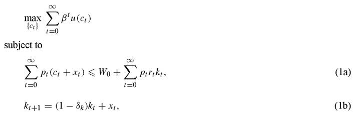
where c_t is the level of consumption, x_t is investment, k_t is the capital stock, p_t is the price of consumption (relative to time 0), and r_t is the rental price of capital, all in

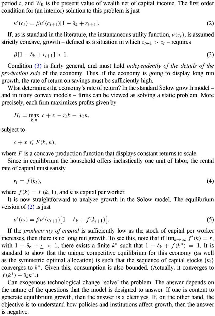
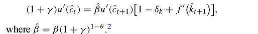
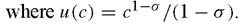
To see this assume that technological progress is labor augmenting. Specifically, as­sume that, at time t, the amount of effective labor is z_t = z( 1+γ)^t. In order to guarantee existence of a balanced growth path we assume that the utility function is isoelastic [see Jones and Manuelli (1990) for details], and given by u(c) = c¹~^θ∕(1 - θ). Let a ^ over a variable denote its value relative to effective labor. Thus, C_t ? c_t∕(z(1 + γ)^t). Inthis case, the balanced growth version of (2) is

Standard arguments show that the equilibrium of this economy converges to a steady state (C, k). Thus, this implies that, asymptotically, consumption is given by c_t = (1 + γ)^tzc. Thus, even though there is equilibrium growth, the growth rate is completely determined by the exogenous increase in labor augmenting productivity.

2.2. A one sector model of equilibrium growth

As we argued before, the critical assumption that results in the economy not growing is that the marginal product of capital is low. The modern growth literature has emphasized the analysis of economies in which the marginal product of capital remains (sufficiently) bounded away from zero. This induces positive long-run growth in equilibrium. As we will show, how fast output grows in these models depends on a variety of factors (e.g., parameters of preferences). Because of this, these models have the property that the rate of growth is determined by the agents in the model.

Throughout, there will be one common theme. This mirrors the point emphasized above, that for growth to occur, the interest rate (either implicit in a planning problem or explicit in an equilibrium condition) must be kept from being driven too low. This follows immediately from the discussion above.

In terms of key features of the environment that are necessary to obtain endogenous growth there is one that stands out: it is necessary that the marginal product of some augmentable input be bounded strictly away from zero in the production of some aug­mentable input which can be used to produce consumption.

Since we are dealing with convex economies, the arguments in Debreu (1954) apply to the environments that we study. Thus, in the absence of distortionary government policies, equilibrium and optimal allocations coincide. Thus, for ease of exposition, we will limit ourselves to analyzing planner’s problems.

The planner’s problem in the basic one sector growth model is given by

As Jones and Manuelli (1990) show, the planner’s solution can be supported as a competitive equilibrium. An extension to multiple goods is presented by Kaganovich (1998) and it is based on similar insights. It is clear that Condition 1 does not rule out decreasing returns to scale.

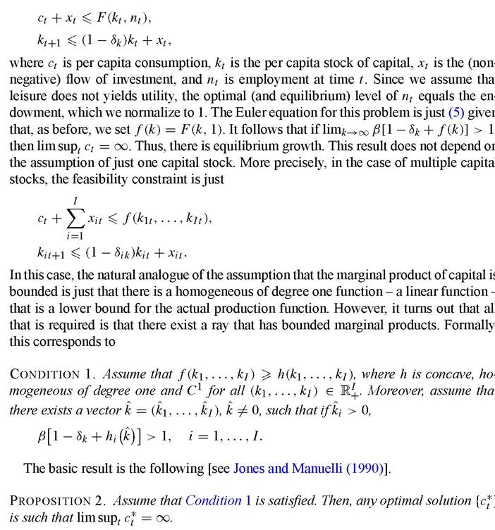
subject to

2.3. Fiscal policy and growth

In this section we describe the effects of taxes and government spending on the long run growth rate. Consider the problem faced by a representative agent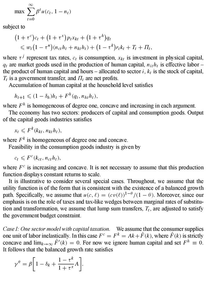

Thus, in this setting, increases in the effective tax on capital, (1 - τ^k)∕(1 + τ^x) un­ambiguously decrease the equilibrium tax rate. Thus, unlike exogenous growth models, government policies affect the growth rate. Moreover, this simple example illustrates that the size of the impact of changes in tax rates on the long run growth rate depends on the intertemporal elasticity of substitution 1 ∕θ. More precisely the elasticity of the growth rate with respect to τ^k is given by

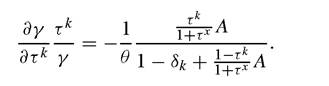
It follows that, other things constant, high values of the intertemporal elasticity of substitution result in large changes in predicted growth rates in response to changes in tax rates. Thus, even an example as simple as this one illustrates that the quantitative predictions of this class of models will heavily depend on the values of the relevant preference (and technology) parameters.

Case II: Physical and human capital: Identical technologies. In this section we as­sume that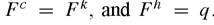This implies that all three goods - investment,

consumption and human capital - are produced using the same technology and, in par­ticular, the same physical to human capital ratio. As in the previous section, τ^k and τ^x do not play independent roles. Thus, to simplify notation, we will set τ^x = 0. How­ever, the reader should keep in mind that increases in the tax rate on capital income are equivalent to increases in the tax rate on purchases of capital goods.

In this case, the balanced growth conditions are

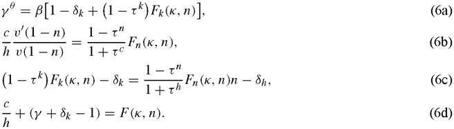
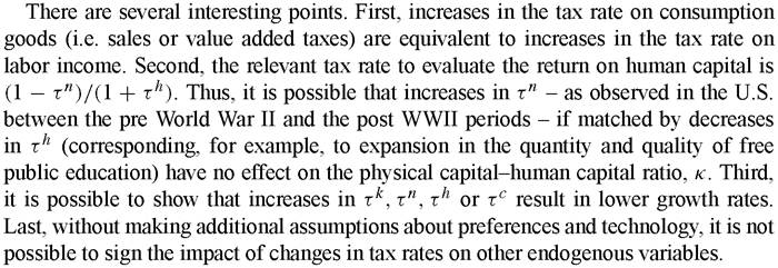
Case III: Physical and human capital: Different factor intensities. In this case, we assume that only human capital is used in the production of human capital. Thus, F^h = A_hn_hh. This is the technology proposed by Uzawa (1964) and popularized in this class of models by Lucas (1988). For simplicity, we only consider capital and labor taxes. The relevant steady state conditions are (6a), (6b), and (6d). However, (6c) becomes

In this version of the model, changes in labor income taxes, reduce growth through their impact on hours worked (relative to leisure). However, if total work time is inelas- tically supplied, i.e. υ(f) ? 1, the growth rate is pinned down by

Thus, in this setting [which corresponds to Lucas (1988) model without the exter­nality, and to Lucas (1990)], taxes have no effect on growth. Increases in the tax rate on capital income simply change physical capital-human capital ratio and they leave the after tax rate of return unchanged.

2.3.1. Quantitative analysis of the effects of taxes

Since the development of endogenous growth theory there have been several studies of the implications of substituting lump-sum taxes for a variety of distortionary taxes. Jones, Manuelli and Rossi (1993) analyze the optimal choice of distortionary taxes in several models of endogenous growth. In the case that physical and human capital are produced using the same technology and labor supply is inelastic, they find that for parameterizations that make the predictions of the model consistent with observations from the U.S., the potential growth effects of drastically reducing (eliminating in most cases) all forms of distortionary taxation is quite high. For their preferred parameteri­zation the increase in growth rates is about 3%. They study a version of the model in which, and the functions F^k and F^h are both of the Cobb-Douglas

variety, but differ in the average productivity of capital. Jones, Manuelli and Rossi esti­mate the capital share parameter to be equal 0.36 in the consumption sector, and to be somewhere in the 0.40-0.50 range in the human capital production sector.^[5] They also allow labor supply to be elastic. Their findings suggest that switching to an optimal tax code result in increases in yearly growth rates of somewhere between 1.5% and 2.0% per year. These are substantial effects.

The third experiment that they consider involves the endogenous determination (by the planner) of the level of government consumption. In this case, they revert back to the one sector version of the model, and they explore not only the consequences of changing the intertemporal elasticity of substitution, but they allow for varying elasticity of sub­stitution between capital and human capital. For their preferred characterization, they also find growth effects of about 2% per year. Moreover, as in the other experiments, the predictions are quite sensitive to the details of the model - in particular, to the choice of the intertemporal elasticity of substitution, and the degree of substitutability between capital and human capital.

Stokey and Rebelo (1995) undertake a thorough review of several models that es­timate the growth impact of tax reform. They argue that in the U.S. tax rates in the post WWII period are significantly higher than in the pre WWII era. This conclusion is based on the increase in the revenue from income taxes as a fraction of GDP in the early 1940s. To reconcile the models with this evidence, they conclude that the human capital share in the production of human capital must be large, and that this sector must be lightly taxed. This description is close to the Case III above and, as argued before, it results in no growth effects.^[6] Thus, in agreement with Lucas (1990) - and using a very similar specification of the human capital production technology - they conclude that changes in tax rates cannot have large growth effects.

This conclusion depends on several assumptions. First, that the U.S. evidence shows an increase in the general level of taxes after WWII. Second, that even if there is a tax increase, the additional revenue is used to finance lump-sum transfers. Third, that the balanced growth path is a good description of the pre and post WWII economy.

Measuring changes in the relevant marginal tax rates is a difficult task. Barro and Sahasakul (1986) using tax records compute average marginal tax rates for the U.S. economy. Their estimates, consistent with the Stokey and Rebelo assumption, show an increase in the 1940s. Even though the evidence about changes in the tax rate consis­tently points to an increase, the implications of this result for the model are not obvious. Consider, first, the uses of tax revenue. If, for example, additional income tax revenues (at the local level) are used to finance local publicly provided goods (e.g., education), then Tiebout-like arguments suggest that the ‘tax effect’ of a tax increase is zero. In the U.S. a substantial increase in government spending corresponds to increases in ex­penditures on education and, hence, the possibility of individuals sorting themselves to buy the ‘right’ bundle of publicly provided private goods cannot be ignored. A second quantitatively important public spending program in the post WWII era is Social Secu­rity. To the extent that benefits are dependent on contributions, the statutory tax rate on labor income used to finance social security overstates the true tax rate.^[7] In this case,

tax payments purchase the right to an annuity whose value is dependent on the pay­ment. Finally, in a model with multiple tax rates an increase in a single tax does not imply, necessarily, a decrease in the growth rate. For the U.S. the evidence on the time path of capital income taxes is mixed. In a recent study, Mulligan (2003) argues that the tax rate on capital income has steadily fallen in the last 50 years. Similarly, McGrattan and Prescott (2003, 2004) find that a decrease in the tax rate on corporate income - one form of capital income - is instrumental in explaining the increase in the value of corporate capital relative to GDP. Overall, we find that the quantitative evidence on the time path of the relevant tax rates to be difficult to ascertain. More work is needed, with an emphasis on matching model and data.

The next section considers the effects of endogenous government spending and tran­sitional effects.

2.3.2. Productive government spending

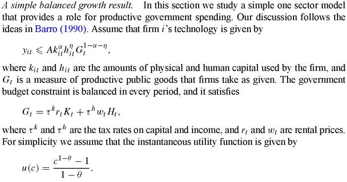
We also assume that the technologies to produce market goods and human capital are identical. In this case, it is immediate to show that the equilibrium is fully described by

where κ is the physical capital-human capital ratio.

Some tedious algebra shows that the growth rate is not a monotonic function of the tax rates. In general, there is no growth when taxes are either too low (not enough public goods are provided) or too high (the private returns to capital accumulation are too low). For intermediate values of the tax rates, growth is positive (if A is sufficiently

high). Thus, in general, increases in tax rates need not result in lower growth if they are accompanied by changes in government spending. Thus, a variant of the model with endogenous government spending (or endogenous taxation and optimally chosen government spending) has potential to reconcile positive growth effects associated with the removal of distortions with the U.S. evidence.

What does the U.S. evidence show? In the U.S. there is a substantial increase in the ratio of government spending to GDP in the post WWII period on the order of 15%. Even ignoring defense related expenditures, the size of the federal government relative to output is close to 5% in the pre WWII period, and it increases steadily in the post war to reach about 20% of income. Of course, not all forms of government spending are productive, but if the trend in the productive component follows the trend in overall spending, ignoring changes in government spending result in biased estimates of the effects of distortions.

The Barro model is silent about the reasons why the desired ratio of (productive) government spending to GDP would increase. For this, it is necessary to have a model of the collective decision making mechanisms which is clearly beyond the scope of this chapter.

Progressive taxes and transition effects. Our discussion of the assumptions that suf­fice for sustained growth clearly shows that homogeneity of degree one is not necessary. In both theoretical and applied work it is common to appeal to linearity in order to ig­nore transitional dynamics [see Bond, Ping and Yip (1996) and Ladron de Guevara, Ortigueira and Santos (1997) for analysis of the dynamics of endogenous growth mod­els]. However, when taking the model to the data, the assumption that the economy is on the balanced growth path may not be appropriate.

In this section we describe the results of Li and Sarte (2001). The basic insight from their model that is relevant for our discussion is that in the presence of heterogeneity in individual preferences and nonlinearities in the tax code, shocks to the tax regime (they consider an increase in the degree of progressivity of the tax code) that ultimately result in a decrease in the growth rate can have basically no effects for several decades.

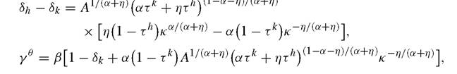
The basic model that they consider is one in which goods are produced according to the following technology

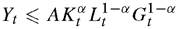
where K_t is capital at time t, L_t is the flow of labor, and G_t is a measure of productive public goods. All individuals have isoelastic preferences given by u(c) = (c^1-θ - 1)/ (1 - θ ), but they differ in their discount factors, β_i. Li and Sarte assume that each type has mass 1 /N, where N is population. The tax code is nonlinear. Given aggregate income Y, and individual income y_i, the tax rate is given by a function τ(z), where z is the ratio of individual to average income. In this application, Lin and Sarte assume that

Note that the case of proportional taxes - the case discussed so far - corresponds to φ = 0. In this setting, higher values of φ are interpreted as corresponding to more progressive tax codes. Individual income is defined as the sum of capital and labor income. Government spending is financed with revenue from income taxes. Li and Sarte show that the equilibrium is the solution to the following system of equations:

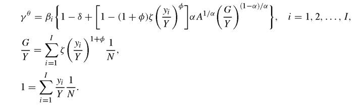
In this model, changes in the progressivity of the tax code affect the rate of return - this is the standard effect - as well as the distribution of income. It is this last effect that generates the slow adjustment. It is possible to show that an increase in φ decreases long run growth, γ.

Li and Sarte explore the dynamic effects of a one time increase in φ that result in a decrease in the growth rate of 1.5%. On impact, output growth increases because since the distribution of income does not adjust immediately, government revenues increase and this, in turn, increases output. As the low discount factor individuals adjust their relative income (an increase in progressivity affects them more than proportionally), government revenue and spending decrease. For parameter values that are designed to mimic the U.S. economy, Li and Sarte find that the half-life of the adjustment is over 40 years. Thus, any test for breaks in the growth rate as suggested by models in which convergence is immediate would conclude (incorrectly) that the tax increase has no effects on growth.

It is difficult to evaluate how appropriate the Li and Sarte model is to study the impact of tax reform in the U.S. economy. However, it casts doubt on the approach by Stokey and Rebelo which ignores transitional dynamics. Models that rely on changes in tax rates that, in turn, affect the distribution of income, are consistent with the view that the effects of those changes are not monotone, and that the full impact may not be felt for decades.

2.4. Innovation in the neoclassical model

One of the things that seems unsatisfactory to many economists in the presentation up to this point is the starkness with which the technological side of the model is described. As we argued above, the key in improving over the Solow model is to explicitly consider decisions made by private agents about investments they make that cause technology to improve. This both endogeneizes the growth process envisaged by Solow and breaks away from another key assumption of the exogenous growth literature, that technolog­ical change happens without any resource cost. But, much of the detail that one thinks about as being an important part of the innovation process seems to be missing from the simple convex models of growth described above. The idea that innovation is carried out by specialized researchers who pass on their newfound knowledge to production line workers is just one example of this. Indeed, one question is whether or not that kind of structure is consistent with convex models of growth at all.

Because of this, in this section we describe a variant of the models presented in the last section that is more directed at identifying innovation as a special activity. The purpose of this exercise is not to fully exhaust the possibilities, but rather to show the reader that more is possible with the class of convex models than one might first think. In particular, since the model we will analyze is convex, standard price taking behavior is consistent with equilibrium behavior. In this sense, the example we will present is similar to the ideas developed by Boldrin and Levine (2002).

There are many models of innovation that do not have convex technology sets [e.g., see the surveys in Barro and Sala-i-Martin (1995) and Aghion and Howitt (1998)]. In this setting, standard price taking behavior is either not consistent with equilibrium in those settings or they must include external effects. Because of this, all policy ex­periments in those models mix two conceptually distinct aspects of policy, the desire to correct for monopoly power and/or external effects and the distortionary effects of ‘wedges’ (e.g., taxes). This, in turn, implies that the answers to questions about the effects of alternative policies on both the incentives to innovate and overall welfare de­pends on the details of the specifications of external effects (e.g., do other researchers learn new innovations for free after one month, or one decade) and/or market power (e.g., is there only one researcher at the frontier and so a monopoly analysis is in order, or are there two, or many). Thus, one thing that a convex model of innovation has to add is answers to some of these questions which are less dependent on those details.

2.4.1. Notation

We will follow the notation above as closely as is possible. We assume that there are two types of labor supply available, researchers and workers. Each individual of each type has his own level of knowledge. We will assume that there is a continuum of identical households each with some researcher time and some worker time to supply to the market. These are given by L₁ researcher hours per household, and L₂ worker hours per household, where L = L₁ + L₂ is total labor supply within the household. We will assume that L₁ and L₂ are fixed, with no ability to move hours between them. (In this sense, it might be easier to think of the household as being made up of L₁ researchers and L2 workers.)

Each household has the level of knowledge H_t that they can use with researcher hours during period t. Thus, if households are symmetric, H_t symbolizes the absolute frontier of what ‘society’ knows at date t. Similarly, the level of knowledge for the average worker hour at date t is denoted by h_t. This will represent the average knowledge of those workers that work in the final goods sector below.

Final consumption at date t is denoted by c_t. We abstract from physical capital to simplify.

Production functions. We will assume that:

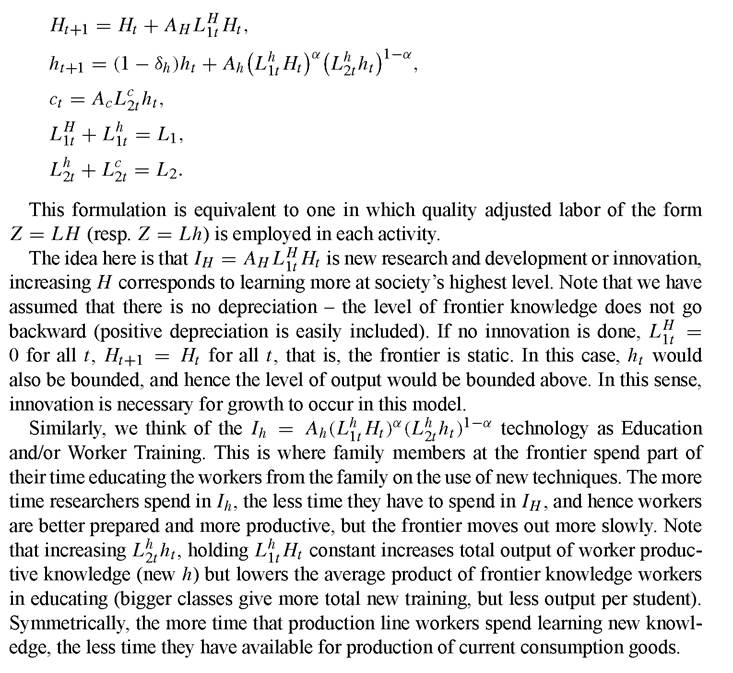
Preferences. We assume that each researcher/worker supplies one unit of labor to the market inelastically and that each has preferences of the form:

This model, although different in detail, shares one com­mon critical feature with those above: linearity in the reproducible factors.

2.4.2. Balanced growth properties of the model

Like many Ak, style models, this one has the feature that it converges to a Balanced Growth Path. Indeed if the initial levels of relative human capitals (H₀ /h₀) are right the economy is on the BGP in every period. Standard techniques can be used to characterize this BGP. After some algebra, we find:

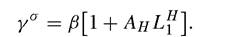
This equation gives γ as a function of the basic parameters σ, β, A_h, and L₁. By construction, the comparative statics of growth rates with respect to the deep parameters of the model are identical to what one would find in an Ak model. The one difference is the inclusion of the endowment of researcher hours, L₁, note that γ is increasing in L₁. That is, if one country had a higher proportion of researchers in its population, output would grow faster.

Since γ does not depend on the other parameters of the model, it can be shown that the only way income taxes affect growth rates here is through their effect on the R&D sector. That is, if we have a linear income tax (at rate τ) either on income generated in all sectors, or on income generated only in the H sector the growth rate will fall to:

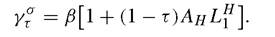
In particular, if income from the h and/or c sectors are taxed, but that from the H sector is not, there are no effects on growth. This is reminiscent of the Lucas (1988) model and the 2-sector model in Rebelo (1991).

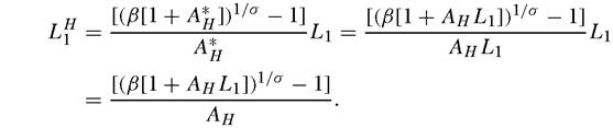
The amount of time spent on R&D on the BGP is given by:

Thus, if we compare two countries with different discount factors, but identical in other respects, the one with the higher β will devote a higher fraction of its researcher time to innovation and a lower percentage to teaching. This causes worker productivity in the consumption sector to be lower at first (and consumption as well), but growing faster and hence, eventually overtaking the low β country.

As a second point, note that increases in A_h do not change γ (and neither do changes in A_c). Thus, in this case, LH is not affected and so the time series of H_t will be iden­tical. This implies that h_t must be higher. Thus, wages of both researchers and workers will be higher. This is similar in spirit to the result in Boldrin and Levine (2002) that improvements in the copying technology raises the value of being an innovator. Since the only ‘copying’ being done here is the passing on of new knowledge to final goods workers, this is analogous in this setting.

These are simple comparative statics exercises which are meant only to show that much intuition about the process of innovation, and its comparative statics properties with respect to incentives can be illustrated in this class of models.

There are many interesting extensions of the analysis that one could imagine. These include heterogeneity among households (e.g., some researcher households, some worker households), the inclusion of uncertainty about the results of researcher time (and the questions that this raises about ex post hold up problems when one researcher is the ‘first’ discoverer), the training of researchers by other researchers when they have different H_t ^,s, the inclusion of more than one good or process, what types of Industrial Organization are possible through decentralizations of the allocation as a competitive equilibrium (e.g., firms specializing in R&D vs. each firm having an R&D division), etc.

But, the reader can see that much of the analysis will go through unchanged. Notable exceptions are when there are assumed to be external effects in the learning process. The simplest example of this here would be to assume that h = H no matter what L⅛ is. In this case, unless this is completely internalized within a firm (i.e., there are no spillovers across firms) the Planner’s problem will not be implementable as a competi­tive equilibrium.

2.4.3. Addinganon-Convexity

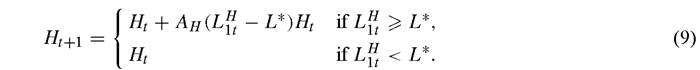
Most models of innovation differ from the one outlined above in that they assume that there is a non-convexity in the innovation technology. There are two ways to include this in the specification above, and the differences between them highlight a key question about innovation.

These are:

and

taking behavior, etc. There are some restrictions on the implicit Industrial Organization in the equilibrium however. For example, for all t it follows that there

can be at most one R&D firm in any equilibrium (or one firm with an R&D division). This, were it true, would cause serious concern for the price-taking assumption in the decentralization.

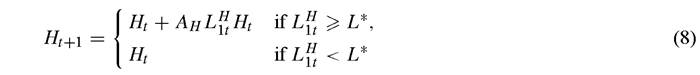
One interesting implication of this model is that whether or not the solution to the planning problem above (without the non-convexity) describes the competitive alloca­tion depends on the size of the country, N. Thus, large countries would, in equilibrium, conduct R&D while small countries would not. Adding in a fourth sector in which researchers in large countries could train researchers in small countries would be a nat­ural extension in which R&D was done in large countries, these researchers train high H workers from small countries (e.g., in Engineering schools), those newly trained ‘re­searchers’ return to their home countries where they subsequently train production line workers, etc.

This description of equilibrium cannot be true for (9), however. Price taking behavior in this setting implies that prices for the rental of new knowledge equal their marginal cost of production. This implies that there is no way to recover the set up cost of re­searchers spending L* hours. Thus, there can be no competitive equilibrium. It follows that there must be some monopoly rent generated somewhere to decentralize any allo­cation. Typically this will be accompanied by inefficiencies and incorrect incentives to conduct R&D.

3.