Fluctuations and growth
3.1. Introduction
In this section we describe existing results on the effects of ‘volatility’, both in technologies and policies, on the long-run growth rate. We start with a brief summary of the empirical research in this area, and we then describe some simple theoretical models that are useful in understanding the empirical results.
We end with the description of some recent work based on the theoretical models but aimed at evaluating their ability to quantitatively match the growth observations. As before, we ignore models based on aggregate non-convexities, and with non-competitive market structures.3.2. Empirical evidence
A relatively small (but growing) empirical literature has tried to shed light on the relationship between ‘instability’ and growth. This literature has concentrated on estimating reduced form models that try to capture, with varying degrees of sophistication, how ‘volatility’ (defined in a variety of different ways) affects long-run growth.
Kormendi and Meguire (1985) is probably the earliest study in this literature. They consider a sample of 47 countries with data covering the 1950-1977 period. Their methodology is to run a cross-country growth regression with the average (over the sample period) growth rate as the dependent variable, and a number of control variables, including the standard deviation of the growth rate (one measure of instability), as well as the standard deviations of policy variables such as the inflation rate and the money supply. Kormendi and Meguire find that the coefficient of the volatility measure (the standard deviation of the growth rate) is positive and significant. Thus, a simple interpretation of their results is that more volatile countries - as measured by the standard deviation of their growth rates - grow at a higher rate.
Grier and Tullock (1989) use panel data techniques on a sample of 113 countries covering a period from 1951 to 1980.
Theirfindings on the effect of volatility on growth are in line with those of Kormendi and Meguire. They find that the standard deviation of the growth rate is positively, and significantly, associated with mean growth rates.Ramey and Ramey (1995) first report the results of regressing mean growth on its standard deviation on a sample of 92 countries as well as a subsample of 25 OECD countries, covering (approximately) the 1950-1985 period. They find that for the full sample the estimated effect of volatility is negative and significant, while for the OECD subsample the point estimate is positive, but insignificant. In order to allow for the variance of the innovations to the growth rate to be jointly estimated with the effects of volatility, Ramey and Ramey posit the following statistical model
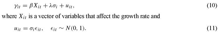
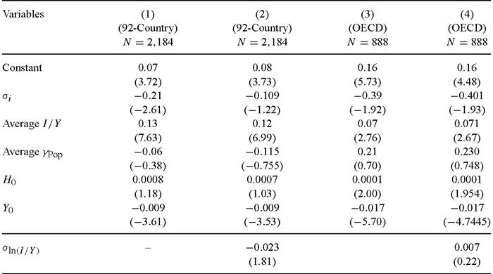
The model is estimated using maximum likelihood. The control variables used were the (average) investment share of GDP (Average I/Y), average population growth rate (Average χpop), initial human capital (measured as secondary enrollment rate, H0), and the initial level of per capita GDP (Y0). They study separately the full sample (consisting of 92 countries) as well as a subsample of 25 OECD (more developed) economies. Their results are reproduced in columns (1) and (3) of Table 1.
For both sets of countries, Ramey and Ramey find that the standard deviation of the growth rate is negatively related to the average growth rate. However, for the OECD subsample, the coefficient is less precisely estimated (even though the point estimate is larger in absolute value). Ramey and Ramey also consider more ‘flexible’ specifications that try to capture differences across countries in the appropriate forecasting equations. Considering the most parsimonious version of their model, the estimated effect of volatility on growth is still positive. However, the strength of the estimated relationship is reversed: for the OECD subsample the point estimate is four times the size of the estimate for the full sample and highly significant.
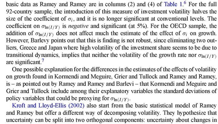
In more recent work, Barlevy (2002) reestimates the Ramey and Ramey model with one change: he adds the standard deviation of the logarithm of the investment-output ratio (σιn(1∕y)) as one of the explanatory variables. Barlevy hypothesizes that this variable can capture non-linearities in the investment function. His results, using the same
Table 1
Growth and volatility I
Note: t-statistics in parentheses.
Source: Columns (1) and (3) - Ramey and Ramey (1995), columns (2) and (4) - Barlevy (2002).
[1] We thank Gadi Barlevy for providing us the estimated coefficient for the control variables.
[1] The point estimates are negative but insignificant.
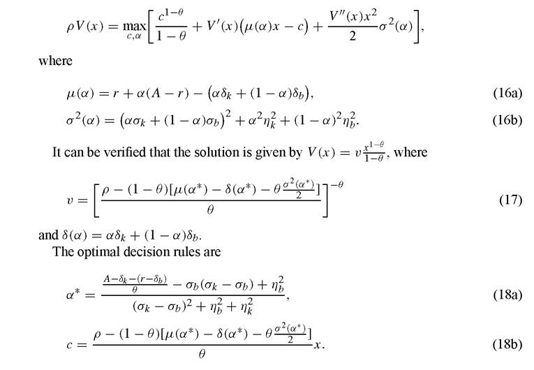
Table 2
Growth and volatility II

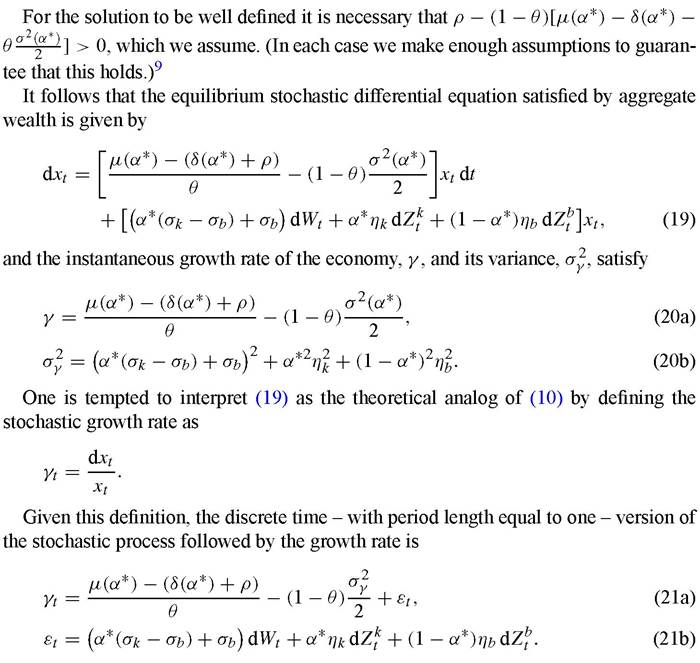
Note: t-statistics in parentheses. Source: Kroft and Lloyd-Ellis (2002).
regime (e.g., expansion-contraction) and fluctuations within a given regime. To this end, they generalize the empirical specification of the Ramey and Ramey statistical model to account for this. They assume that
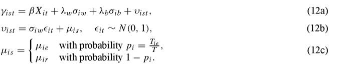
Kroft and Lloyd-Ellis interpret the standard deviation of the random variable μis, σib - which they assumed observed by the economic agents but unobserved by the econometrician - as a measure of variability between regimes, while σiw is viewed as the within-regime variability. Kroft and Lloyd-Ellis estimate their model by maximum likelihood using the same sample as Ramey and Ramey. The results are in Table 2.
The major finding is that the ‘source’ of volatility matters: Increases in σiw - the within phase standard deviation - have a positive impact on growth for the full sample.
For the OECD, the coefficient estimate is still positive but about one third of the size. The effect of the between-phase volatility, σib, is negative in both cases. However, the effects are stronger for the full sample. It is not easy to interpret the phases identified by Kroft and Lloyd-Ellis in terms of a switching model because their estimation procedure assumes that the econometrician can identify whether a particular period corresponds to either a recession or an expansion.[8] Kroft and Lloyd-Ellis also use the same controls as Ramey and Ramey. However, they find that, when the two variances are allowed to differ, none of the control variables is significant. It is not clear why this is the case. One possibility is that the ‘phases’ that they identify are correlated with the control variables (this seems likely situation in the case of investment). Another possibility is that the control variables, in the Ramey and Ramey formulation, capture the nonlinearity associated with the regime shift and that, once the shifts are taken into account, the control variables have no explanatory power. In any case, this illustrates a point that we will come back to: the fragility of the “growth” regressions suggest that better theoretical models are necessary to more provide restrictions that will allow to identify the parameters of interest.The results of Ramey and Ramey and Kroft and Lloyd-Ellis are consistent with the existence of nonlinearities in the relationship between measures of instability and growth. Fatas (2001) estimates a number of different specifications of the relationship between instability and growth. His approach is to run standard cross country regressions. His data set is taken from the most recent version of the Heston-Summers sample and includes 98 countries with information covering the period 1950-1998. His estimates (see Table 3) support the view that the effect of volatility on growth is nonlinear. Using Fatas’ basic estimate - shown in column (1) of Table 3 - the pure effect of volatility is negative with a coefficient of -2.772 indicating that a one standard deviation increase in volatility reduces the growth rate by over 2.5%.
However, the interaction term, corresponding to the variable Volatility ∙ GDP is positive and equal to 0.340. According to these estimates, the net effect of σi on γi for the richest countries in the data is positive and greater than 0.3. For the less developed countries the estimate of the effect of volatility is negative. Columns (2) and (3) use other measures of non-linearity (initial per capita GDP and M3 /Y, a measure of financial development), with similar outcomes: In all cases there is a significant effect, and increases in volatility are less detrimental to growth - and could even have a positive effect - the more developed a country is according to the proxy variables.Martin and Rogers (2000) also study the relationship between the standard deviation of the growth rate and its mean, in a cross section of countries and regions. They study two samples - European regions and industrialized countries - and in both cases they find a negative relationship between σγ and γ. However, when they consider a sample of developing countries the point estimates are positive, but in general insignificant.
It is not easy to explain the differences between Ramey and Ramey, Fatas and Martin and Rogers. The period used to compute the growth rates (1962-1985 for Ramey and Ramey, 1950-1998 for Fatas and 1960 to 1988 for Martin and Rogers), and the
Table 3
Growth and volatility III
| Independent variable | (1) | (2) | (3) |
| Volatility (σi) | -2.772 | -1.700 | -0.270 |
| (0.282) | (0.645) | (0.091) | |
| GDP per capita (1960) | -2.229 | -1.856 | -0.953 |
| (0.235) | (0.422) | (0.220) | |
| Human capital (1960) | 0.037 | 0.040 | 0.026 |
| (0.015) | (0.018) | (0.017) | |
| Average investment share of GDP | 0.083 | 0.143 | 0.120 |
| (0.013) | (0.021) | (0.024) | |
| Average population growth rate | -0.624 | -0.562 | -0.465 |
| (0.153) | (0.205) | (0.465) | |
| Volatility ∙ GDP | 0.340 (0.036) | - | - |
| Volatility ∙ GDP (1960) | - | 0.212 (0.082) | - |
| - | - | 0.004 (0.001) | |
| R2 | 0.77 | 0.58 | 0.57 |
Note: Sample 1950-1998.
Robust standard errors in parentheses. Source: Fatas (2001).
set of less developed countries included (68 in Ramey and Ramey’s study, and 72 in Martin and Rogers’) are fairly similar. The two studies differ on their definition of the growth rate (simple averages in the Ramey and Ramey and Fatas papers, and estimated exponential trend in Martin and Rogers), and in the variables that are used as controls. However, it is somewhat disturbing that what appear, in the absence of a theory, as ex-ante minor differences in definitions can result in substantial differences in the estimates.
Siegler (2001) studies the connection between volatility in inflation and growth rates and mean growth for the pre 1929 period. Specifically, he uses panel data methods for a sample of 12 (presently developed) countries over the 1870-1929 period. He finds that volatility and growth are negatively correlated, and this finding is robust to the inclusion of standard growth regression type of controls.
Dawson and Stephenson (1997) estimate a model similar to (10) and (11) applied to U.S. states. They use the average (over the 1970-1988 period) growth rate of gross state product per worker for U.S. states as their growth variable, and its standard deviation as a measure of volatility. In addition, they include in their cross-sectional regression the standard (in growth regressions) control variables (investment rate, initial level of gross state product per worker, labor force growth rate, and initial human capital). Dawson and Stephenson find that volatility has no impact on the growth rate, once the other effects are included. Unfortunately, they do not report the ‘raw’ correlation between mean growth and its standard deviation. Thus, it is not possible to determine if the lack of significance is due to the use of controls, or is a more robust feature of U.S. states growth performance.
Mendoza (1997) differs from the previous studies in terms of his definition of instability. Instead of the standard deviation of the growth rate, which, in general, is endogenous, he identifies instability with the standard deviation of a country’s terms of trade. He estimates a linear model using a cross section of countries and finds a negative relationship between instability and growth. His sample is limited to only 40 developed and developing countries, and it only covers the period 1971-1991.
A fair summary of the existing results is that there is no sharp characterization of the relationship between fluctuations and growth. Variation across studies in samples or specifications yield fairly different results. Moreover, the findings do not seem robust to details of how the statistical model is specified.
Are the empirical findings of the channel through which uncertainty affects growth more robust? Unfortunately, the answer is negative. Ramey and Ramey find that volatility - measured as the standard deviation of the growth rate - does not affect the investment-output ratio. More recently, Aizenman and Marion (1999) find that volatility is negatively correlated with investment, when investment is disaggregated between public and private. Fatas estimates a non-linear model of the effect of volatility on investment. He finds that increases in volatility decrease investment in poor countries, but that the opposite is true in high income countries. Thus his findings are consistent with the view that changes in volatility affect mean growth rates through (at least partially) their impact upon investment decisions.
How should these empirical results be interpreted? Even though it is tempting to take one’s preferred point estimate as a measure of the impact of fluctuations (or business cycles) on growth there are two problems with this approach. First, the empirical estimates are not robust to the choice of specification of the reduced form. Second, and more important in our opinion, is that from the point of view of policy design, the relevant measures of volatility is the - in general unobserved - volatility in policies and technologies. In most models, the growth rate (and its standard deviation) are endogenous variables and, as usual, the point estimate of one endogenous variable on another is at best difficult to interpret. One way of contributing to the interpretation of the empirical results is to study what simple theoretical models predict for the estimated relationships. In the next section we present a number of very simple models to illustrate the possible effects of volatility in fundamentals on mean growth. In the process, we find that it is very difficult to interpret the empirical findings. To put it simply, there are theoretical models that - depending on the sample - do not restrict the sign of the estimated coefficient of the standard deviation of the growth rate on its mean. Moreover, the sign and the magnitude of the coefficient is completely uninformative to determine the effect of volatility on growth.
3.3. Theoretical models
The analysis of the effect of uncertainty on growth can be traced to the early work of Phelps (1962), and Levhari and Srinivasan (1969) who studied versions of the stochastic consumption-saving problem that are similar to the linear technology versions of endogenous growth models. More recently, Leland (1974), studies a stochastic Ak model, and he shows that the impact of increased uncertainty on the consumption/output ratio depends on the size of the coefficient of risk aversion.
Even in deterministic versions of models that allow for the possibility of endogenous growth, existence of equilibria (and even optimal allocations) requires strong assumptions on the fundamentals of the economy [see Jones and Manuelli (1990) for a discussion]. At this point, there are no general results on existence of equilibrium in stochastic versions of those models. In special cases, most authors provide conditions under which an equilibrium exists [see Levhari and Srinivasan (1969), Mendoza (1997), Jones, Manuelli and Siu (2003), Jones et al. (2003) for various versions]. A recent, more general result is contained in de Hek and Roy (2001). These authors consider fairly general utility and production functions, but limit themselves to i.i.d. shocks. It is clear that more work is needed.
In what follows, we will describe a general linear model and we will use it to illustrate the predictions of the theory for the relationship between mean growth rates and their variability. To simplify the presentation we switch to a continuous time setting. In order to obtain closed-form solutions we specialize the model in terms of specifying preferences and technology. Moreover, we will limit ourselves to i.i.d. shocks. Generalizations of these assumptions are discussed in the section that presents quantitative results.
3.4. A simple linear endogenous growth model
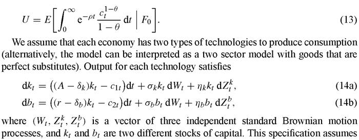
We begin by presenting a stochastic analog of a standard Ak model with a ‘twist’. Specifically, we consider the case in which there are multiple linear technologies, all producing the same good. In order to obtain closed-form results we specify that the utility of the representative household is given by
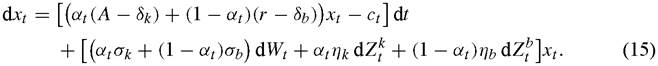
that each sector is subject to an aggregate shock, Wt, as well as sector (or technology) specific shocks, Zj.
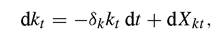
To simplify the algebra, we assume that capital can be costlessly reallocated across technologies, and we denote total capital by χt ? kt + bt. Setting (without loss of generality) kt = αtxt (and, consequently bt = (1 - αt)xt) it follows that total capital evolves according to
Given the equivalence between equilibrium and optimal allocations in this convex economy, we study the solution to the problem faced by a planner who maximizes the utility of the representative agent subject to the feasibility constraint. Formally, the planner solves
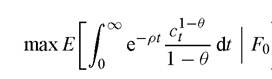
subject to (15).
Let the value of this problem be V(x). Then, it is standard to show that the solution to the planner’s problem satisfies the Hamilton-Jacobi-Bellman equation
This simple model driven by i.i.d. shocks has a stark implication: the growth rate is
i.i. d. and is independent of other endogenous (or exogenous) variables, except through the joint dependence on the error term. Using panel data, it is relatively easy to reject this implication. This, however, is not an intrinsic weakness of this class of models. The theoretical setting can be generalized to include serially correlated shocks and a nonlinear structure, which could account for “convergence” effects, and would provide a role for lagged dependent variables. However, generalizing the theoretical model comes at the cost of not being able to discuss the impact of different factors on the growth rate, except numerically.
[1] In endogenous growth models existence of an equilibrium is not always guaranteed. The main problem is that with unbounded instantaneous utility and production sets, utility can be infinite. Fora discussion of some conditions that guarantee existence see Jones and Manuelli (1990) and Alvarez and Stokey (1998). The key issue is that the return function is unbounded above when 0 < θ < 1, and unbounded below if θ > 1. In this setting, it can be shown that c > 0 is equivalent to ensuring boundedness.
What is the (simple) class of model that we study useful for? We view the class of theoretical models that we present as more appropriate to discuss the implications of the theory for cross section regressions since, in this case, the constant μ(α ')-(δα ')+ρ') -
2
(1 - θ)-γ can be correlated with other variables like the investment-output ratio.
Even though there is a formal similarity between (21) and (10)-(11), the theoretical model suggests that the simple approach that ignores that the same factors that affect σγ, also influence the true value of β in (10) can result in incorrect inference. Alternatively, the “deep parameters” are not the means and the standard deviation of the growth rates. They are the means and standard deviations of the driving stochastic processes. In terms of those parameters, the “true” model is non-linear.
Whether the model in (21) implies a positive or negative relationship between fluctuations and growth depends on the sources of shocks. At this general level it is difficult to illustrate this point, but we will come back to it in the context of specific examples.
It is not obvious how to define the investment ratio in this model. The change in cumulative investment in k, Xk,is given by
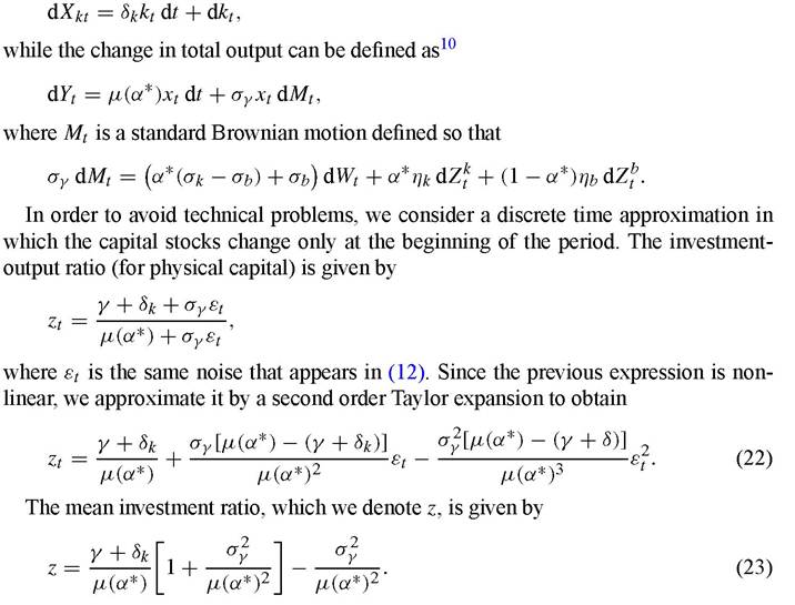
[1] This is not the only possible way of defining output. It assumes that the economy two sectors (or technologies). However, another interpretation of this basic framework considers bt as bonds, and kt as the only real stock of capital. We will be precise about the notion of output in each application.
Given this approximation, the model implies that the covariance between the growth rate and the investment-output ratio is
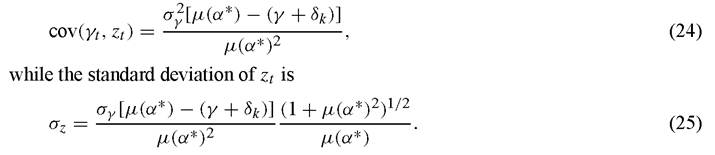
Simple algebra shows that, given that the existence condition (17) is satisfied, cov(γt, zt) > 0. Thus, in a simple regression, the investment ratio has to appear to affect positively growth. At this general level it is more difficult to determine if high σz economies are also high γ economies. The problem is that there are a number of factors that jointly affect γ and σz. In order to be more precise, it is necessary to be specific about the sources of heterogeneity across countries. We will be able to discuss the sign of this relationship in specific contexts.
We now use this ‘general’ model to discuss - in a variety of special cases - the connection between the variability of the growth rate of output and its mean.
3.4.1. Case 1: An Ak model
Probably the simplest model to illustrate the role played by differences in the variability of the exogenous shocks across countries is the simple Ak model. Even though it is a special case of the model described in the previous section, it is useful to describe the technology in a slightly different way. Let the feasibility constraint for this economy be given by

The left-hand side of this condition is the accumulated flow of output until time t, and the right-hand side is the accumulated uses of output, consumption and investment. The law of motion of capital is
where δk is the depreciation rate. Expressing the economy’s feasibility constraint in flow form, and substituting in the law of motion for physical capital, the resource constraint satisfies

The planner’s problem - which coincides with the competitive equilibrium in this economy - is to maximize (13) subject to (26). This problem resembles the more general model we introduced in the previous section if we set ηb = σb = ηk = 0, and 
σk = σyA.
In addition, we need to make sure that the “b” technology is not used in equilibrium. A simple way of guaranteeing this is to view r - δb as endogenous, and to choose it so that, in equilibrium, α* = 1; that is, all of the investment is in physical capital. It is immediate to verify that this requires
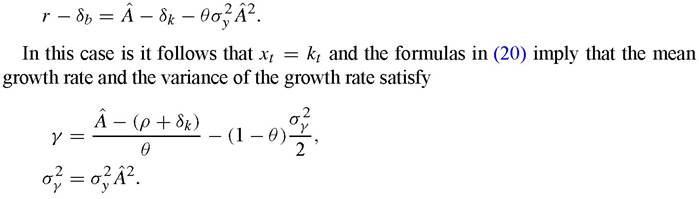
This result, first derived by Phelps (1962) and Levhari and Srinivasan (1969), shows that, in general, the sign of the relationship between the variance of the technology shocks, σy2, and the growth rate is ambiguous:
• If preferences display less curvature than the logarithmic utility function, i.e. 0 < θ < 1, increases in σy are associated with decreases in the mean growth rate, γ.
• If θ > 1, increases in σy are associated with increases in the mean growth rate, γ.
• In the case in which the utility function is the log (this corresponds to θ = 1) there is no connection between fluctuations and growth.
The basic reason for the ambiguity of the theoretical result is that the total effect of a change in the variance of the exogenous shocks on the saving rate - and ultimately on the growth rate - can be decomposed in two effects that work in different directions:
• An increase in the variance of the technology makes acquiring future consumption less desirable, as the only way to purchase this good is to invest. Thus, an increase in variance of the technology shocks has a substitution effect that increases the demand for current (relative to future) consumption. This translates into a lower saving and growth rates.
• On the other hand, an increase in the variability of the exogenous shocks induces also an income effect. Intuitively, for concave utility functions, the fluctuations of the marginal utility decrease with the level of consumption. Thus, the (negative) effect of fluctuations is smaller when consumption is high. This income effect increases savings, as this is the only way to have a ‘high’ level of consumption (i.e. to spend more time on the relatively flat region of the marginal utility function).
The formula we derived shows that the relative strength of the substitution and income effects depends on the degree of curvature of the utility function: if preferences have less curvature than the logarithmic function, the substitution effect dominates and increases in the variance of the exogenous shocks reduce growth. If the utility of the representative agent displays more curvature than the logarithmic function, the income effect dominates and the relationship between fluctuations and growth is positive.
In this simple economy, the variance of the technology shock, σ2, and the variance of the growth rate of output, σ2, coincide up to scale factor A.11 If one views the differences across countries as due to differences in σ2,12 the theoretical model implies that the true regression equation is very similar to the one estimated in the empirical studies. The only difference is that the theory implies that it is σ2, and not σγ, that enters the right hand side of (10). If we use this model to interpret the results of Ramey and Ramey (1995), one must conclude that the negative relationship between mean growth and its standard deviation is evidence that preferences have less curvature than the logarithmic utility, i.e. 0 < θ < 1. On the other hand, the Kormendi and Meguire (1985) findings suggest that θ > 1.
In this simple example, the mean investment ratio - the appropriate version of (23) - is
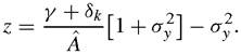
As was pointed out in the previous section, the covariance between the investmentratio and the growth rate is positive. In this example, the appropriate version of (25) is
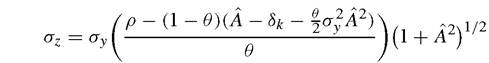
Inthis case, increases in σy are associated with increases (decreases) in σz if θ ) 1. Thus, if θ < 1, the higher the (unobserved) variance of the technology shocks (σ2), the higher the (measured) variances of both the growth rate, σγ2, and the investment rate, σ2, and the lower the mean growth rate. Moreover, in this stochastically singular setting the standard deviation of the growth rate and the investment rate are related (although not linearly). Thus, this simple model is consistent with the findings of Barlevy (2002) that the coefficient of σz is estimated to be negative, and that its introduction reduces the significance of σγ.
This simple model cannot explain the apparent non-linearity in the relationship between mean and standard deviation of the growth rate process which, according to Fatas (2001), is such that the effect of σγ on γ is less negative (and can be positive) for high income countries. In order to account for this fact it is necessary to increase the degree of heterogeneity, and to consider non-linear models.
Finally, the model can be reinterpreted as a multi-country model in which markets are incomplete and the distribution of the domestic shocks - the productivity shocks - is common across all countries.11 12 [9] [10] [11] More precisely, consider a market structure in which
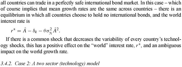
In the previous model, the variance of the growth rate is exogenous and equal to the variance of the technology shock. This is due, in part, to the assumption that the economy does not have another asset that can be used to diversify risk. In this section we present a very simple two-technology (or two sector) version of the model in which the variance of the growth rate is endogenously determined by the portfolio decisions of the representative agent. The main result is that, depending on the source of heterogeneity across countries, the relationship between σγ and γ need not be monotone. In particular, and depending on the source of heterogeneity across countries, the model is consistent with increases in σγ initially associated with increases in γ, and then, for large values of σγ, with decreases in the mean growth rate.
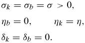
To keep the model simple, we assume that the second technology is not subject to shocks, and we ignore depreciation. Thus, formally, we assume that ηb = σb = ηk = 0. However, unlike the previous case, the “safe” rate of return r satisfies
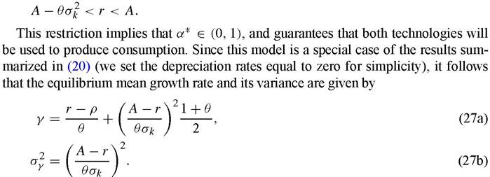
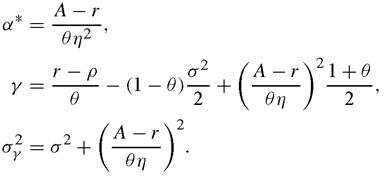
How can we use the model to interpret the cross country evidence on variability and growth? A necessary first step is to determine which variables can potentially vary across countries. In the context of this example, a natural candidate is the vector (A, r,σk). Before we proceed, it is useful to describe the connection between γ and σγ implied by the model. The relationship is - taking a discrete time approximation -
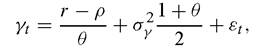
εt = σγωt, ωt ~ N(0, 1).
It follows that if the source of cross-country differences are differences in (A, σk) the model implies that - independently of the degree of curvature of preferences - the relationship between σγ2 and γ is positive. To see why increases in σk result in such a positive association between the two endogenous variables σγ and γ, note that, as σk rises, the economy shifts more resources to the safe technology (α* decreases) and this, in turn, results in a decrease in the variance of the growth rate (which is a weighted average of the variances of the two technologies). Since the ‘risky’ technology has higher mean return than the ‘safe’ technology, the mean growth rate decreases. The reader can verify that changes in A have a similar effects.
If the source of cross-country heterogeneity is due to differences in r, the implications of the model are more complex. Consider the impact of a decrease in r. From (27b) it follows that σγ2 increases and this tends to increase γ. However, as (27a) shows, this also decreases the growth rate, as it lowers the non-stochastic return. The total effect depends on the combined impact. A simple calculation shows that
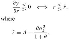
To better understand the implications of the model consider a “high” value of r; in particular, assume that r > r. A decrease in r reduces σγ and, given that r > r,it results in an increase in γ. Thus, for low σγ (high r) countries, the model implies a positive relationship between γ and σγ. If r < r, decreases in the return to the safe technology still increase σγ, but, in this region, the growth rate decreases. Thus, in (σγ,γ) space the model implies that, due to variations in r, the relationship between σγ and γ has an inverted U-shape.
Can this model explain some of the non-linearities in the data? In the absence of further restrictions on the cross-sectional joint distribution of (A, r, σk) the model can accommodate arbitrary patterns of association between σγ and γ. If one restricts the source of variation to changes in the return r the model implies that, for high variance countries, variability and growth move in the same direction, while for low variance countries the converse is true. If one could associate low variance countries with relatively rich countries, the implications of the model would be consistent with the type of non-linearity identified by Fatas (2001).
3.4.3. Case 3: Aggregate vs. sectoral shocks
The simple Ak model that we discussed in the previous section is driven by a single, aggregate, shock. In this section we consider a two sector (or two technology) economy to show that the degree of sectoral correlation of the exogenous shocks can affect the mean growth rate. To capture the ideas in as simple as possible a model, we specialize the specification in (14) by considering the case
Note that, in this setting, there is an aggregate shock, Wt, which affects both sectors (technologies) while the A sector is also subject to a specific shock, Z,k. Using the formulas derived in (18) and (20) it follows that the relevant equilibrium quantities are
As before, it is useful to think of countries as indexed by (A, r, σ, η). Since changes in each of these parameters has a different impact, we analyze them separately.
• An increase in σ. The increase in the standard deviation of the economy-wide shock affects both sectors equally, and it does not induce any ‘portfolio’ or sectoral reallocation of capital. The share of capital allocated to each sector (technology) is independent of σ. Since increases in σ increase σγ (in the absence of a portfolio reallocation, this is similar to the one sector case), the total effect of an increase in σ is to decrease the growth rate if 0 < θ < 1, and to increase it if θ > 1.
• A decrease in r. The effect of a change in r parallels the discussion in the previous section. It is immediate to verify that a decrease in r results in an increase in σγ. However, the impact on γ is not monotonic. For high values of r, decreases in r are associated with increases in γ, while for low values the direction is reversed. Putting together these two pieces of information, it follows that the predicted relationship between σγ and γ is an inverted U-shape, with a unique value of σγ (a unique value of r) that maximizes the growth rate.
• An increase in η. This change increases the ‘riskiness’ of the A technology and results in a portfolio reallocation as the representative agent decreases the share of capital in the high return sector (technology). The change implies that σγ and γ decrease. Thus, differences in η induce a positive correlation between mean and standard deviation of the growth rate.
• What is the impact of differences in the degree of correlation between sectoral shocks. Note that the correlation between the two sectoral shocks is
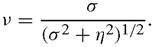
In order to isolate the impact of a change in correlation, let’s consider changes in (σ, η) such that the variance of the growth rate is unchanged. Thus, we restrict (σ, η) to satisfy

for a given (fixed) σγ. It follows that the correlation between the two shocks and the growth rate are
Thus, lower correlation between sectors (in this case this corresponds to higher σ) unambiguously lower mean growth. If countries differ in this correlation then the implied relationship between σγ and γ need not be a function; it can be a correspondence. Put it differently, the model is consistent with different values of γ associated to the same σγ.
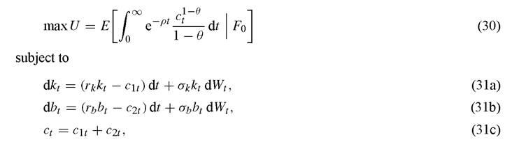
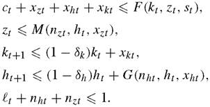
3.5. Physical and human capital
In this section we study models in which individuals invest in human and physical capital. We consider a model in which the rate of utilization of human capital is constant. Even though the model is quite simple it is rich enough to be consistent with any estimated relationship between σγ and γ.
We assume that output can be used to produce consumption and investment, and that market goods are used to produce human capital. This is equivalent to assuming that the production function for human capital is identical to the production function of general output. The feasibility constraints are
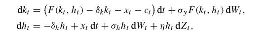
where (W- Zt ) is a vector of independent standard Brownian motion variables, and F is a homogeneous of degree one, concave, function. As in the previous sections, let xt = kt + ht denote total (human and non-human) wealth. With this notation, the two feasibility constraints collapse to
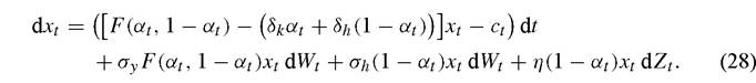
As in previous sections, the competitive equilibrium allocation coincides with the solution to the planner’s problem. The planner maximizes (13) subject to (28). The
Hamilton-Jacobi-Bellman equation corresponding to this problem is

where
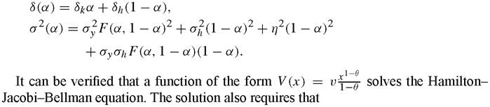
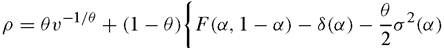
where a is given by
For any homogeneous of degree one function F, the solution is a constant a. Moreover, a does not depend on v. Existence requires υ > 0, and this is just a condition on the exogenous parameter that we assume holds.14
The growth rate and its variance are given by

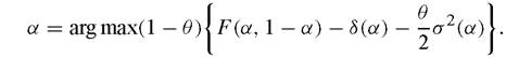
It follows that, for the class of economies for which the planner problem has a solution (i.e. economies for which v > 0, and γ > 0), the conjectured form of V(x) solves the HJB equation, for any homogeneous of degree one function F. However, in order to make some progress describing the implications of the theory, it will prove convenient to specialize the technology and assume that F is a Cobb-Douglas function given by

The next step is to characterize the optimal share of wealth invested in physical capital, a, and how changes in country-specific parameters affect the mean and standard deviation of the growth rate. It turns out that the qualitative nature of the solution depends on the details of the driving stochastic process. To simplify the algebra, we assume that the human capital technology is deterministic (i.e. σh = η = 0), and that both stocks of capital (physical and human) depreciate at the same rate (δk = δh). As
[1] This is just the stochastic analog of the existence problem in endogenous growth models.
[1] InthecaseoftheCobb-Douglasproductionfunctiontherearetwovaluesof α thatsatisfy F (α*') = 1∣Oθy.
[1] The reader can check that, in this case, the solution α*' = ω does not satisfy the second order condition.
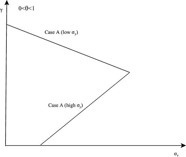
Figure 1. The mapping σγ and γ [0 < θ < 1].
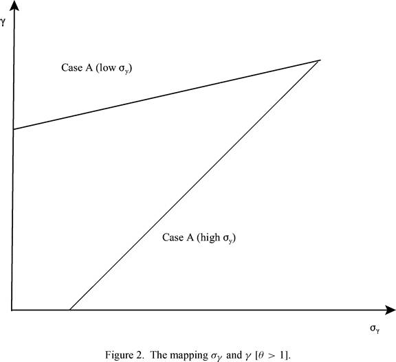
between σγ and γ.[17] In the case of θ > 1, the size of θ matters only to determine which branch is steeper. In both cases A and B the relationship between the standard deviation of the growth rate and the mean growth rate is upward sloping. However, the low σ∕2-branch is flatter (and lies above) the high σ∕2-branch (see Figure 2).
Since we have studied a very simple version of this class of models, it does not seem usefUl to determine the relevance of each branch by assigning values to the parameters. In ongoing work, we are studying more general versions of this setup. However, even this simple example suggests that some caution must be exercised when interpreting the empirical work relating the variability of the growth rate and its mean. Unless one can rule out some of these cases, theory gives ambiguous answers to the question that motivated much of the literature, i.e. do more stable countries grow faster? Moreover, the theoretical developments suggest that progress will require to estimate structural models rather than reduced form equations.
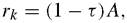
3.6. The opportunity cost view
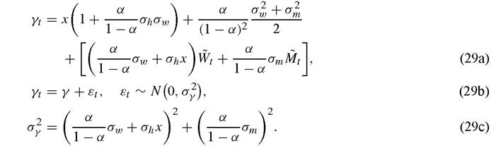
So far the models we discussed emphasize the idea that increases in the variability of the driving shocks can have positive or negative effects upon the growth rate depending on the relative importance of income and substitution effects. An alternative view is that recessions are “good times” to invest in human capital because labor - viewed as the single most important input in the production of human capital - has a low opportunity cost. In this section we present a model that captures these ideas. The model implies that the time allocated to the formation of human capital is independent of the cycle.[18] [19] It also implies that shocks to the goods production technology have no impact on growth, but that the variability of the shock process in the human capital technology decreases growth. As before, we concentrate on a representative agent with preferences described by (13). The goods production technology is given by where nt is the fraction of the time allocated to goods production, kt is the stock of physical capital, and ht is the stock of human capital. The variable zt denotes a stationary process. To simplify the theoretical presentation we assume that capital depreciates fully. Thus, goods consumption is limited by Human capital is produced using only labor in order to capture the idea that the opportunity cost of investing in human capital is market production. The technology is summarized by where, as before, Wt is a standard Brownian motion.[20] Given that the problem is convex[21] the competitive allocation solves the planner’s problem. It is clear that, given ntht, physical capital will be chosen to maximize net output. This implies that consumption is or, taking a discrete time approximation, Equation (29a) completely summarizes the implications of the model for the data. There are several interesting results. To simplify the notation, we will refer to Wt as the aggregate shocks and to Mt as the idiosyncratic component of the productivity shock in the goods sector. • The share of the time allocated to human capital formation - the engine of growth in this economy - is independent of the variability of the technology shock in the goods sector, as measured by (σw, σm). • High (σw, σm) economies are also high growth economies. Thus, if cross-country differences in σγ are mostly due to differences in (σw, σm), the model implies a positive correlation between the standard deviation of the growth rate and mean growth. • It can be shown that increases in σh result in decreases in σhx. Thus, if countries differ in this dimension the model also implies a positive relationship between σγ and γ. • In the model, investment in physical capital (as a fraction of output) is α, independently of the distribution of the shocks. Thus, there is no sense that a regression that shows that variability does not affect the rate of investment provides evidence against the role of shocks in development. • This lack of (measured) effect on both physical and human capital investment should not be interpreted as evidence against the proposition that incentives for human or physical capital accumulation matter for growth. It is easy enough to include a tax/subsidy to the production of human capital - consider a policy that affects B - and it follows that this policy affects growth. 3.7. More on government spending, taxation, and growth In this section we consider a simple Ak model in which a government uses distortionary taxes to finance an exogenously given stochastic process for government spending. Our analysis follows Eaton (1981).[22] The representative household maximizes utility - given by (13) - by choosing consumption and saving in either capital or bonds. However, given that tax policy is exogenously fixed, it is not the case that the rate of return on bonds is risk free. On the contrary, since the government issues bonds to make up for any difference between revenue and spending it is necessary to let the return on bonds to be stochastic. The representative household problem is where kt is interpreted as capital and bt as bonds. As before, it is possible to simplify the analysis by using wealth as the state variable. Let χt ? kt + bt. With this notation, the single budget constraint is given by c The set of feasible allocations is the set of stochastic process that satisfy 23 This, of course, depends on the fact that the solution to the individual agent problem is such that bonds and capital are held in fixed proportions. it follows that, Equation (34a) summarizes the impact of both technology and fiscal shocks on the expected growth rate. Consider first the impact of variations in the tax regime on the relationship between the variability of the growth rate, σγ, and the average growth rate. If technology shocks, σ, are the main source of differences across countries in the standard deviation of the growth rate, then high variability countries are predicted to be low mean countries if 1 - θ - τ' + θg' > 0; that is, if a country has a relatively low tax rate on the stochastic component of income. This, would be the case if the base of the income tax allowed averaging over several periods. On the other hand, countries with relatively high tax rates on the random component of income display a positive relationship between the mean and the variance of their growth rates. As in more standard models, high capital income tax countries (high τ countries) have lower average growth. Differences across countries in the average size of the government, g in this notation, have no impact on growth. Finally, cross country differences in the fraction of the random component of income consumed by the government, g', induce a positive correlation between γ and σγ. This is driven by the negative impact that increases in g' have on mean growth, and the equally negative effect that those changes have on σγ. Thus, high g' countries display low average growth rates, which do not fluctuate much.24 3.8. Quantitative effects In this section we summarize some of the quantitative implications various models for the relationship between variability and growth. Unlike the theoretical models described above, the quantitative exercises concentrate on the role of technology shocks in models with constant - relative to output - government spending. Mendoza (1997) studies an economy in which the planner solves the following problem: subject to [1] The impact of some variables in the previous analysis differs from the results in Eaton (1981) since our specification of the fiscal policy allows the demand for bonds (as a fraction of wealth) to be endogenous, and driven by changes in the tax code. Eaton assumes that the share of bonds, 1 - α in our notation, is given, and some tax must adjust to guarantee that demand and supply of bonds are equal. where At is a measure of assets and pt is interpreted as the terms of trade. Since this equation can be rewritten as where kt = At∕pt is the stock of assets (capital) measured in units of consumption, and rt+1 = Rt pt∕pt+1 is the random rate of return, it is clear that Mendoza’s model is a stochastic version of an Ak model. The rate of return, rt is assumed to be Iognormally distributed with mean and variance given by It follows that the standard deviation of the growth rate is σγ = σ. Mendoza studies the effect of changing σ from 0 to 0.15, holding μr constant. To put the exercise in perspective, the average across countries of the standard deviations of the growth rate or per capita output in the Summers-Heston dataset is 0.06. Thus, the model is calibrated at a fairly high level of variability. The results depend substantially on the assumed value of θ. For θ = 1/2, the non-stochastic growth rate is 3.3%. If σ = 0.10, it decreases to 2.5%, while it is 1.6% when σ = 0.15. For θ = 2.33 (Mendoza’s preferred specification), the growth rate increases from 0.7% to 0.9% in the given range. For other values of the coefficient of risk aversion, the impact of uncertainty is also small. In summary, unless preferences are such that the degree of intertemporal substitution is large, increases in rate of return uncertainty have a small impact on mean growth rates. Jones et al. (2003) analyze the following planner’s problem: subject to For their quantitative exercise, they specify the following functional forms: The model is calibrated to match the average growth, in a cross section of countries, and its standard deviation. Jones et al. (2003) consider the impact of changing the standard deviation of the shock, st, from 0 to 0.15. The impact on the growth rate depends on the curvature of the utility function. For preferences slightly less curved than the log, the model predicts an increase in the growth rate of 0.7% an annual basis, while for θ = 1.5, the effects is an increase in the growth rate of 0.25%. However, the model predicts that σγ - which is endogenous - is unusually high (of the order of 0.10) unless θ ≥ 1.5. Thus, Jones et al. (2003) obtain results that are quite different from those of Mendoza (1997). There are two important differences between the models: First, while Mendoza (1997) assumes that shocks are i.i.d., Jones et al. (2003) set the first order correlation parameter, p, to 0.95. Second, while Mendoza assumes a constant labor supply, Jones et al. allow for the number of hours to vary with the shock. In order to disentangle the effect of the components of the standard deviation of the technology shock, Jones et al. vary σε and p in a series of experiments, where σs = σε∕(1 — p2)1/2, where σε is the standard deviation of the innovations. They find that changes in σε appear quantitatively more important than those and p. Moreover, they also find that the relative variability of hours worked is very sensitive to the precise value of θ. Economies with high θ, and lower σγ in their specification, also display substantially less variability in hours worked. Even though it is not possible to determine on the basis of these two results which is the critical feature that accounts for the differences between the results obtained by Mendoza (1997) and Jones et al. (2003), it seems that the assumption of a flexible supply of hours - which determines the rate of utilization of human capital - is a leading candidate.[25] In a series of papers, Krebs (2003a, 2003b) explores the impact of changes in uncertainty in models where markets are incomplete. Building on the work of de Hek (1999), Krebs (2003a) studies the impact of shocks to the depreciation rate of the capital stock. Even though he assumes that instantaneous utility is logarithmic, he finds that increases in the standard deviation of the shock, decrease growth rates. This result is driven by the “location” of the shocks, and it does not require market incompleteness.[26] Quantitatively, Krebs (2003a) finds that an increase in the standard deviation of the growth rate from 0 to 0.15 (a fairly large value relative to the world average) reduces growth from 2.13% to 2.00%. If the variability is increased to 0.20 the growth rate drops to 1.5%. However, these values are substantially higher than those observed in international data.[27] The theoretical analysis of the impact of different forms of uncertainty on the growth of the economy is still in its infancy. Simple existing models suggest that the sign of the relationship between the variability of a country’s growth rate and its average growth rate is ambiguous. Thus, theoretical models that restrict more moments can help in understanding the effect of fluctuations on growth and welfare. The few quantitative studies that we reviewed have produced conflicting results. It seems that the precise nature of the shocks, their serial correlation properties and the elasticity of hours with respect to shocks all play a prominent role in accounting for the variance in predicted outcomes. Much more work is needed to identify realistic and tractable models that will be capable of confronting both time series and cross country observations. 4.


More on the topic Fluctuations and growth:
- Aghion Philippe, Durlauf Steven N. (eds.). Handbook of Economic Growth. Volume 1. Part A. North-Holland,2005. — p. 1-1060, 2005
- Learning Objectives
- Czech Republic
- Learning Objectives
- SUMMARY
- All populations fluctuate in size
- The Schumpeterian approach
- Historical Phases, Territorial Fluctuations, and International Standing
- In the previous chapters we have focused on the effects of aggregate volatility and aggregate productivity or trade shocks on long-run growth, taking volatility as being largely exogenous.
- Some populations exhibit logistic growth, a pattern in which abundance increases rapidly at first and then stabilizes at a population size known as the carrying capacity, the maximum population size that canbe supported indefinitely by the environment