All populations fluctuate in size

Another characteristic of the sheep population in Tasmania is seen in all populations: their size rises and falls over time, illustrating the third and most common pattern of population growth, population fluctuations.

growth. If, for example, the growth of a population exactly matched a logistic curve, the population would not be said to fluctuate. But if population abundances rose above and fell below those expected in exponential growth (as in the cattle egret) and logistic growth (as in the Tasmanian sheep), the population would be said to fluctuate.

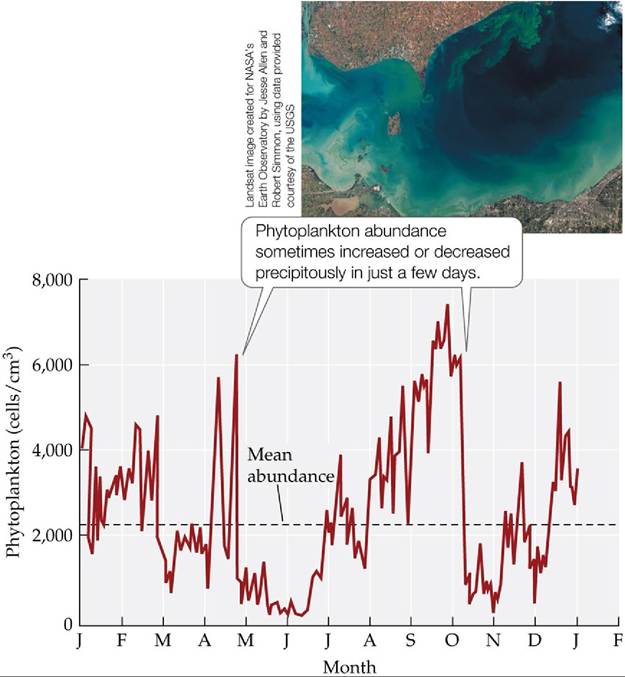
FIGURE 10.6 PopulationFluctuations Variationinphytoplanktonabundanceinwater samples taken from Lake Erie during 1962, showing fluctuations above and below the overall mean abundance of 2,250 cells per cubic centimeter. The inset shows an October 2011 phytoplankton “bloom” (a rapid increase in phytoplankton numbers) in the lake. (After C. C. Davis. 1964. Limnol Oceanogr 9: 275-283.) View larger image

In some cases, population fluctuations are relatively small (as seen in Figure

10.5). In other cases, the number of individuals in a population can explode at certain times, causing a population outbreak (FIGURE 10.7). As we saw in Figure 10.2A, the biomass of the comb jelly Mnemiopsis increased 1,000-fold during a 2-year outbreak in the Black Sea. Rapid variations in population sizes over time have also been observed in many terrestrial systems, especially in insects. Census data for the bordered white moth (Bupalus piniarius) collected from 1882 to 1940 in a German pine forest showed that the densities reached during outbreaks were up to 30,000 times as great as the lowest density observed.

FIGURE 10.7 PopulationscanExplodeinNumbers When conditions are favorable, a population outbreak can occur in which the numbers of individuals increase very rapidly. The cockroaches covering the kitchen in this exhibit from the National Museum of Natural History represent the number that could have been produced by a single pregnant female in a few generations. View larger image

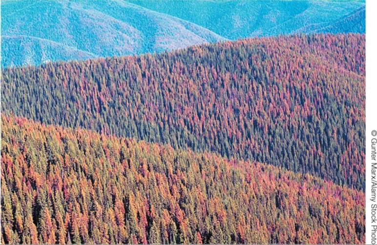
FIGURE 10.8 Consequences of an Insect Outbreak This aerial view shows the red foliage of lodgepole pine (Pinus contorta) trees killed by an outbreak of mountain pine beetles in British Columbia, Canada. View larger image

Many different factors can cause the size of a population to fluctuate. The increase in zooplankton populations in the Black Sea in the early 1980s probably occurred because their prey (phytoplankton) had increased in abundance (see Figure 10.2). Then, in 1991, zooplankton numbers plummeted, probably because of the spectacular increase in the abundance of their predator (Mnemiopsis) during the previous 2 years. The rapid changes in phytoplankton abundance in Lake Erie shown in Figure 10.6 could reflect changes in a wide range of environmental factors, including nutrient supplies, temperature, and predator abundance.

Analyzing the factors important to population fluctuations can also help identify the factors important to disease outbreaks. In 1993, dozens of people in the Four Corners region of the southwestern United States (where New Mexico, Arizona, Colorado, and Utah intersect) became sick with flu-like symptoms and shortness of breath, and 60% of them died within a few days of becoming ill. No one had seen this combination of symptoms before. An outbreak of a lethal, previously unknown disease appeared to be in progress, and there was no cure or successful treatment. The U.S. Centers for Disease Control (CDC) quickly identified the disease agent as a new strain of hantavirus carried by the deer mouse (Peromyscus maniculatus). Seeking more information about the new disease, now known as hantavirus pulmonary syndrome, or HPS, the CDC contacted ecologists who had been studying mouse populations in the Southwest. Examination of deer mouse specimens collected between 1979 and 1992 revealed that the virus had been present in the area for more than 10 years prior to the outbreak. Why, then, did the outbreak of HPS occur in 1993 and not before?

To address this question, ecologists used data on the abundances of Peromyscus species collected since 1989 at the nearby Sevilleta National Wildlife Refuge. These data showed that the densities of several Peromyscus species had increased 3- to 20-fold between 1992 and 1993. Next, a series of satellite images was used to develop an index of how much plant matter was available as food for Peromyscus at different times. When that index was compared with precipitation data, the results suggested that unusually high rainfall from September 1991 through May 1992 had led to enhanced plant growth in spring 1992 (FIGURE 10.9). In turn, the enhanced plant growth produced abundant food for rodents (seeds, berries, green plant matter, arthropods), which allowed mouse populations to increase in size by 1993—the year of the HPS outbreak.

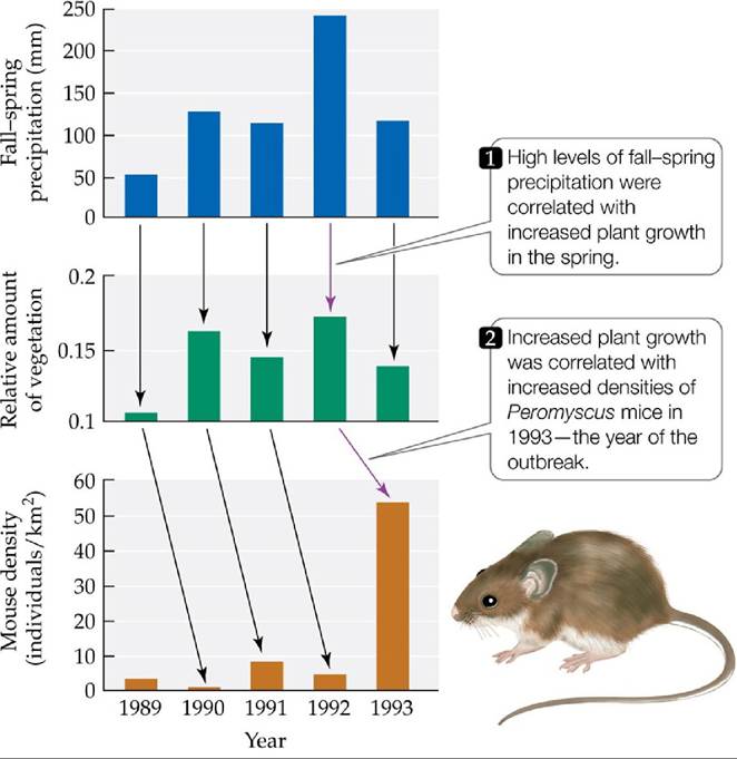
FIGURE 10.9 From Rain to Plants to Mice Theoutbreakofhantaviruspulmonary syndrome in the southwestern United States in 1993 may have been caused by a series of interconnected events.

Rodents shed hantavirus in their urine, feces, and saliva; hence, high mouse numbers, which led to increased mouse-human contact, were thought to be the cause of the 1993 outbreak. The actual risk to people varies greatly with location and depends on such factors as habitat type (which can influence mouse movements), microclimate (e.g., in arid regions, nearby areas often experience very different amounts of rainfall), and local food abundance. Overall, we now know enough about HPS to predict periods of heightened risk to human populations, but more remains to be learned about whether these factors create predictable population cycles in mice and the hantavirus disease. Let's now turn to what ecologists know about the factors important in producing population

cycles.