Small populations are at much greater risk of extinction than large populations

The size of a population has a strong effect on its risk of extinction. For example, Jones and Diamond (1976) studied extinction in bird populations on the Channel Islands, located off the coast of California.

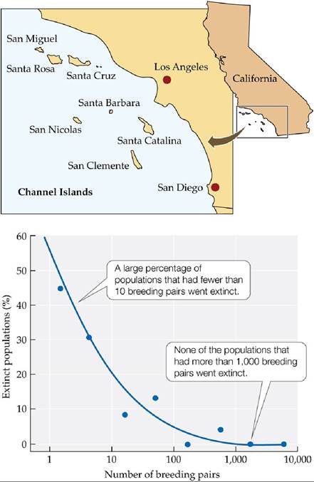
FIGURE 10.12 Extinction in Small Populations AmongbirdpopulationsontheChannel

Islands, the percentage of populations that went extinct declined rapidly as the number of breeding pairs in the population increased.

Assume that a population is at high risk (>30%) of extinction. Use the graph to estimate the total number of breeding pairs the population should have to

reduce its risk of extinction to 5%.

(After H. L. Jones and J. M. Diamond. 1976. Condor 78: 526-549.) View larger image

These findings for birds have been confirmed in many other groups of organisms. Overall, field data indicate that the risk of extinction increases greatly when population size is small. But what are the factors that place small populations at risk?

When populations are small, they reduce what is called effective population size, or the number of individuals that can contribute offspring to the next generation.

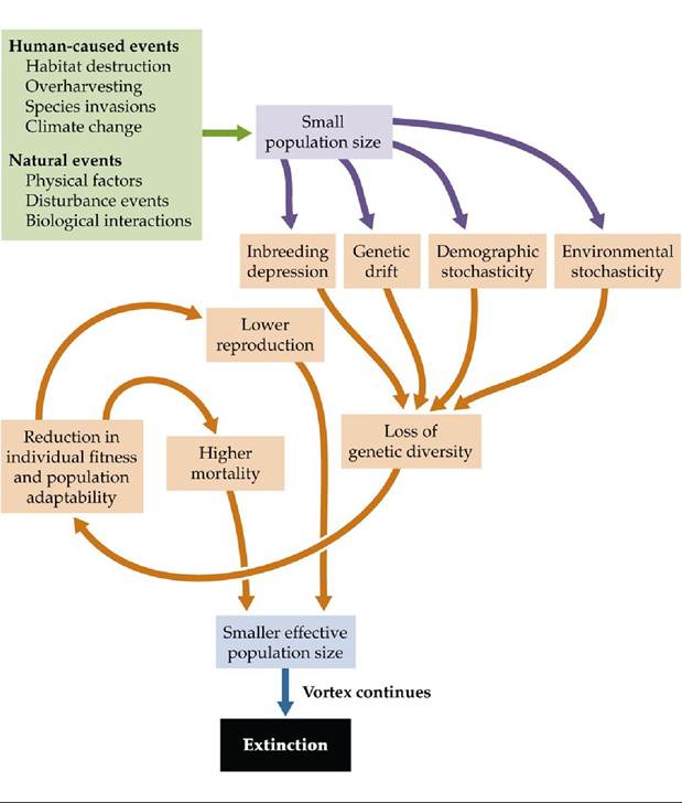
FIGURE 10.13 ExtinctionVortex Human-caused and natural events can reduce the effective population size of species, resulting in the loss of genetic diversity, and eventually leading to population- and species-level extinctions. View larger image

Risk from Genetic Factors

Small populations can encounter problems associated with genetic drift and inbreeding depression, processes that reduce genetic diversity and the fitness of individuals and the adaptability of populations (see Figure 10.13). Recall from Concept 6.2 that genetic drift is the process by which chance events influence which alleles are passed on to the next generation. Genetic drift can occur in many ways, including chance events that determine whether individuals reproduce or die. Imagine, for example, that an elephant walks through a population of ten small plants, 50% of which have white flowers (genotype aa) and 50% of which have red flowers (AA). If the elephant happens to crush more red-flowered than white-flowered plants, then by chance alone, there will be more copies of the a allele than of the A allele in the next generation. This scenario is just one of many possible examples of how genetic drift can cause allele frequencies to change at random from one generation to the next.

Genetic drift has little effect on large populations, but in small populations it can cause losses of genetic variation over time. For example, if genetic drift causes the frequency of two alleles (e.g., A and a) to change at random in each generation, one allele may eventually increase to a frequency of 100% (reach fixation), while the other is lost (see Figure 6.7).

In addition, small populations can show a high frequency of inbreeding (mating between related individuals). Inbreeding is common in small populations because after several generations at a small population size, most of the individuals in the population will be closely related to one another (to see why, answer Review Question 3). Inbreeding tends to increase the frequency of homozygotes, including those that have two copies of a harmful allele. Thus, like genetic drift, inbreeding depression can lead to the loss of genetic diversity, reducing individual fitness and hence population growth rates.

The combined negative effects of genetic drift and inbreeding depression appear to have reduced the fertility of male lions that live on the floor of the Ngorongoro Crater, Tanzania (FIGURE 10.14). From 1957 to 1961, there were 60 to 75 lions living in the crater, but in 1962 an extraordinary outbreak of biting flies caused all but 9 females and 1 male to die. Seven males immigrated into the crater in 1964-1965, but no further immigration has occurred since that time. The population has increased in size since the 1962 crash. From 1975 to 1990, for example, the population fluctuated between 75 and 125 individuals. However, genetic analyses indicated that all these individuals were descendants of just 15 lions (Packer et al. 1991). In a population of 15 individuals, genetic drift and inbreeding depression have powerful effects. Those effects appear to be the reason why the crater population has less genetic variation and more frequent sperm abnormalities than the large population of lions found nearby on the Serengeti Plain. In such a situation, all is not necessarily lost: in some cases, populations in decline because of drift and inbreeding have been “rescued” by introducing a small number of individuals from other, more genetically diverse populations (see Figure 23.16).

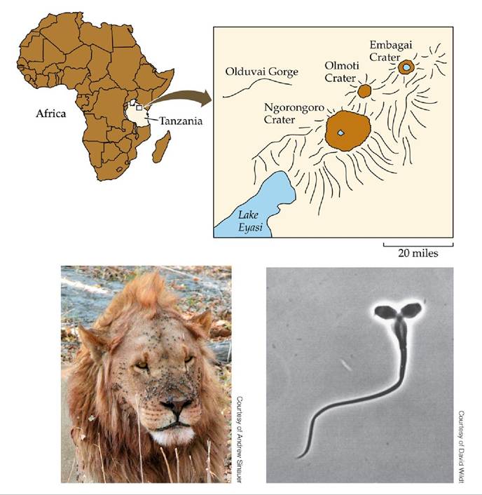
FIGURE 10.14 APlagueofFlies In 1962, the population of lions in the 260-km² (100- square-mile) Ngorongoro Crater of Tanzania was nearly driven to extinction by a catastrophic outbreak of biting flies similar to those on the face of this male. Lions became covered with

infected sores and eventually could not hunt, resulting in many deaths. In the population that descended from the few survivors, genetic drift and inbreeding depression have led to frequent sperm abnormalities, such as this “two-headed” sperm. View larger image

Risk from Demographic Factors

A second factor important to the loss of genetic diversity, and ultimately extinction, in small populations is that of demographic Stochasticity, or the fluctuations in population size as the result of chance differences among individuals in reproduction and survival (see Figure 10.13). For example, for an individual, survival and reproduction are all-or-nothing events: an individual either survives or it does not, and it either reproduces or it does not. At the population level, we can transform such all-or-nothing events into a probability that survival or reproduction will occur. For example, if 70 out of 100 individuals in a population survive from one year to the next, then (on average) each individual in the population has a 70% chance of survival.

In a small population, however, demographic stochasticity can result in outcomes that differ from what such averages would lead us to expect. Consider a population of ten individuals for which previous data indicate that, on average, each individual has a 70% probability of surviving from one year to the next. However, many chance events—such as whether an individual is struck by a falling tree—can cause the percentage of individuals that actually do survive to be higher or lower than 70%. For example, if six of the ten individuals experienced (the ultimate) “bad luck” and died in chance mishaps, the observed survival rate (40%) would be much lower than the expected 70%.

In contrast, when the population size is large, there is little risk of extinction from demographic stochasticity. The fundamental reason for this has to do with laws of probability. You are, for example, much more likely to receive zero heads if you toss a fair coin 3 times than if you toss the same coin 300 times. Similarly, when we consider the demographic fates of individuals, we can see that chance events are much more likely to cause reproductive failure or poor survival in small populations than in large populations. If each individual in a population has a 33% chance of producing zero offspring, then if there are two individuals in the population, there is an 11% chance (0.33 ? 0.33 = 0.33² = 0.11) that no offspring will be produced—driving the population to extinction in one generation. Although demographic stochasticity could cause a population of 30 individuals to fluctuate in size (perhaps leading to eventual extinction), there is essentially no chance (0.33³⁰) that it could cause the population to go extinct in a single generation.

Demographic stochasticity is also one of several factors that can cause small populations to experience Allee effects. Allee effects occur when the population growth rate decreases as the population density decreases, perhaps because individuals have difficulty finding mates at low population densities (FIGURE 10.15). This phenomenon reverses the usual assumption that population growth rates tend to increase as population density decreases (see Figure 11.12). Allee effects can be disastrous for small populations. If demographic stochasticity or any other factor decreases the population size, Allee effects can cause the population growth rate to drop, which causes the population size to decrease even further in a downward spiral toward extinction.

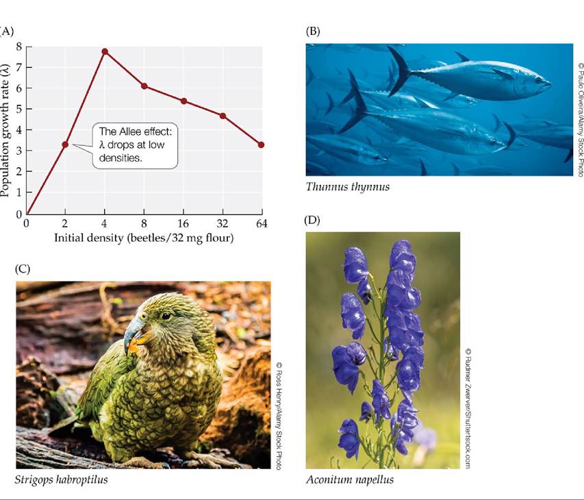
FIGURE 10.15 Allee Effects Can Threaten Small Populations Alleeeffectsoccurwhen the growth rate of a population decreases as population density decreases. (A) In laboratory experiments with the flour beetle Tribolium, population growth rates reached their lowest point at the lowest initial density. Allee effects can be important in animals such as (B) bluefin tuna (Thunnus thynnus), which form schools whose protective or early warning systems function poorly at small population sizes. Allee effects are also important in species in which individuals have difficulty finding mates at low population densities; there are many such species, including (C) kakapos (Strigops habroptilus) and (D) monkshood (Aconitum napellus). (A after F. Courchamp et al. 1999. Trends Ecol Evol 14: 405-410.) View larger image

Risk from Environmental Variation

Finally, environmental Stochasticity can cause declines in genetic diversity and ultimately extinction of small populations (see Figure 10.13). Environmental Stochasticity refers to erratic or unpredictable changes in the environment. In the simulations described above (see Figure 10.11), we've already seen that (1)

variation in environmental conditions that causes fluctuations in population growth rates can lead to population size fluctuations and thus an increased risk of extinction, and (2) such environmental variation is more likely to cause extinction when the population size is small. Many species face such risks from environmental stochasticity. For example, census data on female grizzly bears (Ursus arctos horribilis) in Yellowstone National Park showed that the average population growth rate varied from year to year. Despite the fact that the population tends to grow in size, researchers using a mathematical model found that random variation in environmental conditions could place the Yellowstone grizzly population at high risk of extinction, especially if the population size were to drop to 40 females or less from its 1997 level of 99 females (FIGURE 10.16).

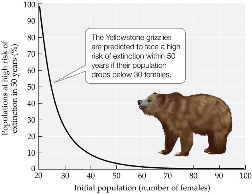
FIGURE 10.16 EnvironmentaistochasticityandpopuIationSize Thisgraphplotsthe risk that the Yellowstone grizzly bear population will be close to extinction in 50 years against the population size (number of females). By studying 39 consecutive years of census data, researchers found that the average population growth rate of Yellowstone grizzlies could lead to explosive growth if it remained constant from year to year. The risk of extinction increased dramatically when random variation in environmental conditions dropped the population size to 40 females or less. (After W. F. Morris and D. F. Doak. 2002. Quantitative Conservation Biology: Theory and Practice of Population Viability. Oxford University Press/Sinauer: Sunderland, MA.) View larger image

Environmental stochasticity differs from demographic stochasticity in a fundamental way. Environmental stochasticity refers to changes in the average birth or death rate of a population that occur from one year to the next. These year-to-year changes reflect the fact that environmental conditions vary over time, affecting all the individuals in a population: sometimes there are good years and sometimes there are bad years. In demographic stochasticity, the average (population-level) birth and death rates may be constant across years, but the actual fates of individuals differ because of the random nature of whether each individual reproduces or not, and survives or not.

Populations also face risks from extreme environmental events such as floods, fires, severe windstorms, or outbreaks of disease or natural enemies. Even though they occur rarely, such natural catastrophes can eliminate or drastically reduce the size of populations that otherwise would seem large enough to be at little risk of extinction. For example, disease outbreaks have resulted in mass mortality in populations of sea urchins (up to 98% of the individuals in some populations) and Baikal seals (killing about 2,500 of a population of 3,000 seals).

Environmental stochasticity also played a key role in the extinction of the heath hen (Tympanuchus cupido cupido). This bird was once abundant from Virginia to New England. By 1908, hunting and habitat destruction had reduced its population to 50 birds, all on the island of Martha's Vineyard, where a 1,600- acre reserve was established for its protection. Initially, the population thrived, increasing in size to 2,000 birds by 1915. A population of 2,000 may seem large enough to be nearly “bulletproof” against the problems that threaten small populations, including genetic drift and inbreeding, demographic stochasticity, and environmental stochasticity. However, a series of disasters struck between 1916 and 1920, including a fire that destroyed many nests, unusually cold weather, a disease outbreak, and a boom in the number of goshawks (a predator of heath hens). Because of the combined effects of these events, the heath hen population dropped to 50 birds by 1920 and never recovered. The last heath hen died in 1932.

With the benefit of hindsight, we can see that heath hens were vulnerable in 1915 because they all lived in a single population. More typically, members of a species are found in metapopulations, which are often isolated from one another by regions of unsuitable habitat. You can read more about metapopulation dynamics in Concept 9.4.

A Case Study Revisited

A Sea in Trouble

In the late 1980s and early 1990s, the Black Sea ecosystem was under severe duress from the combined effects of eutrophication and invasion by the comb jelly Mnemiopsis leidyi, as described in the Case Study. Although Mnemiopsis numbers declined sharply in 1991, they rose steadily again from 1992 to 1995, and then remained high for several years—at about 250 g per square meter, which translates to over 115 million tons of Mnemiopsis throughout the Black Sea. The situation did not look promising. But by 1999, matters were different: the Black Sea was showing signs of

recovery.

The events that set the stage for the recovery of the Black Sea actually began prior to the first onslaught of Mnemiopsis. In the mid- to late 1980s, the amounts of nutrients added to the Black Sea began to level off. From 1991 to 1997, nutrient inputs declined, probably because of hard economic times in former Soviet Union countries coupled with national and international efforts to reduce nutrient inputs. The reduction had rapid effects: after 1992, phosphate concentrations in the Black Sea declined, phytoplankton biomass began to fall, water clarity increased, and zooplankton abundance increased. Mnemiopsis still posed a threat, however, as evidenced by its high biomass and by falling anchovy catches from 1995 to 1998 (see Figure 10.2). Scientists and government officials were gearing up to combat the threat from Mnemiopsis when the problem was inadvertently solved by the arrival of another comb jelly, the predator Beroe (FIGURE 10.17).

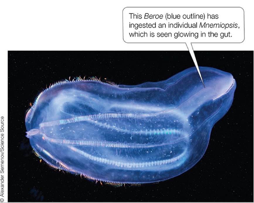
FIGURE 10.17 InvaderversusInvader Another invasive comb jelly species, the predator Beroe, brought Mnemiopsis under control, thus contributing to the recovery of the Black Sea ecosystem. View larger image

Beroe arrived in 1997. Like Mnemiopsis, Beroe probably reached the Black Sea in the ballast water of ships from the Atlantic. Beroe feeds almost exclusively on Mnemiopsis. It is such an effective predator that within 2 years of its arrival, Mnemiopsis numbers plummeted (see Figure 10.2A). Following the sharp decline in Mnemiopsis, the Black Sea population of Beroe also crashed, presumably because it depended on Mnemiopsis for food. The fall of Mnemiopsis led to a rebound in zooplankton abundance (which had dropped again from 1994 to 1996) and to increases in the

population sizes of several native jellyfish species. In addition, after the Mnemiopsis population crashed, there was an increase in the anchovy catch and in field counts of anchovy egg densities. Overall, the decline of Mnemiopsis helped to improve the condition of the Black Sea ecosystem, including the fisheries on which people depend for food and income.

Connections in Nature

From Bottom to Top, and Back Again

The decrease in nutrient inputs by human activities and the control of Mnemiopsis by Beroe had rapid beneficial effects on the entire Black Sea ecosystem. The speed and magnitude of the ecosystem’s recovery provide a source of hope, suggesting that it may be possible to solve large problems in other aquatic communities. Note, however, that ecologists rarely attempt to solve such problems by deliberately introducing new predators, such as Beroe, because such introductions can also have unanticipated negative effects.

The details of the fall and rise of the Black Sea ecosystem also illustrate two important types of causation in ecological communities: bottom-up and top-down controls. The fall of the Black Sea ecosystem began when increased nutrient inputs led to problems associated with eutrophication: increased phytoplankton abundance, increased bacterial abundance, decreased oxygen concentrations, and fish die-offs. The effect of adding nutrients to the Black Sea illustrates bottom-up control, which occurs when the abundance of a population is limited by nutrient supply or food availability. In this case, prior to nutrient enrichment, phytoplankton abundance—and thus the abundance of food for other organisms—was limited by the supply of nutrients.

Ecosystems are also affected by top-down control, which occurs when the abundance of a population is limited by predators. Recent evidence indicates that early steps in the decline of the Black Sea ecosystem were driven not only from the bottom up (by eutrophication), but also from the top down, by overfishing (Daskalov et al. 2007). Starting in the late 1950s, overfishing caused sharp drops in the abundances of predatory fishes. As predatory fish populations declined, their prey, planktivorous (plankton-eating) fishes, increased in number (FIGURE 10.18A). In turn, the increase in planktivorous fishes was associated with declining numbers of zooplankton and increasing numbers of phytoplankton (FIGURE 10.18B,C), suggesting possible top-down control. Later, the arrival of the voracious predator Mnemiopsis also had a top-down effect, altering many key features of the ecosystem (e.g., zooplankton abundance, phytoplankton abundance, fish abundance). Top-down control also seems to have influenced ecosystem recovery: it took another predator, Beroe, to rein in Mnemiopsis. In reality, as in the Black Sea, bottom-up and top-down controls interact to shape how ecosystems work. We'll return to bottom-up and top-down controls in Units 5 and 6, where we consider these important topics in more detail.

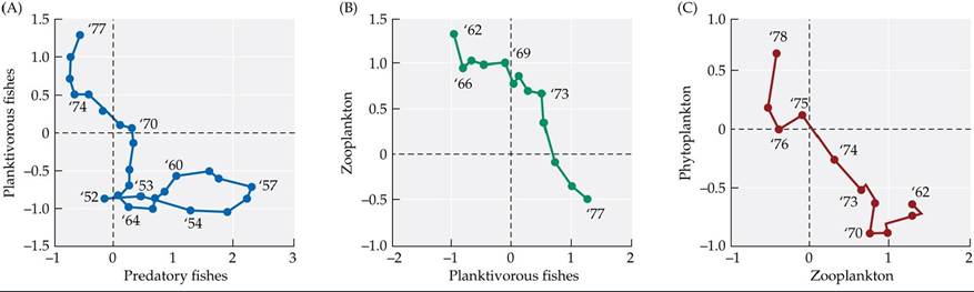
FIGURE 10.18 Ecosystem Changes in the Black SeaAbundanceindicesof(A) planktivorous and predatory fishes, (B) zooplankton and planktivorous fishes, and (C) phytoplankton and zooplankton. In each graph, the organisms whose abundance is plotted on the ó-axis are eaten by the organisms whose abundance is plotted on the x-axis. (Planktivorous fishes eat both zooplankton and phytoplankton, but they have a greater effect on zooplankton abundance than on phytoplankton abundance.) Numbers on the plots indicate years, beginning in 1952. In the abundance indices, data are standardized to have a mean of 0 and a variance of 1.

Referring to (A), describe predatory and planktivorous fish abundance from 1952 to 1957. Next, summarize how abundances of phytoplankton, zooplankton, planktivorous fishes, and predatory fishes changed in the 1970s. Finally, convert your summary of abundance changes in the 1970s into a chain of feeding relationships, where arrow thickness indicates the strength of each relationship (see Figure 9.19, in which similar chains are shown for Alaska). Is the chain you drew more similar to that in Alaska pre-1990 or that in Alaska in the late 1990s? Explain.

(After G. M. Daskalov et al. 2007. Proc NatlAcad Sci USA 104: 10518-10523. © National Academy of Sciences, U.S.A.) View larger image