Size, openness and growth: Empirical evidence
In this section, we review the empirical evidence on trade openness and growth, as well as the empirical evidence on country size and growth. We then argue that the two are fundamentally linked, because both openness and country size determine the extent of the market.
Thus, their impact on growth cannot be evaluated separately. Then we estimate a specification for the determination of growth as a function of market size (itself a function of both country size and trade openness), derived directly from the model presented in Section 2. Our estimates, which are consistent with a growing body of evidence on the role of scale for growth, also provide strong support for our specific model. In particular, we show that the costs of smallness can be avoided by being open. In other words, the impact of size on growth is decreasing in openness, or, conversely, the impact of openness on growth falls as the size of countries increases. This evidence suggests that the extent of the market is an important channel for the realization of the growth gains from trade.3.1. Trade and growth: a review of the evidence
The literature on the empirical evidence of trade and growth is vast and a comprehensive survey is beyond the scope of this article. In this subsection, we simply summarize some of the salient results from recent studies in this literature, in order to set the stage for a discussion of the more specific issue of market size and growth.
The fact that openness to trade is associated with higher growth in post-1950 crosscountry data was until recently subject to little disagreement.[354] Whether openness is measured by indicators of trade policy openness (tariffs, nontariff barriers, etc.) or by the volume of trade (the ratio of imports plus exports to GDP), numerous studies document this correlation. For example, Edwards (1998) showed that, out of nine indicators of trade policy openness, eight were positively and significantly related to TFP growth in a sample of 93 countries.
Dollar (1992) argued that an indicator of openness based on price deviations was positively associated with growth. Ben-David (1993) demonstrated that a sample of countries with open trade regimes displays absolute convergence in per capita income, while a sample of closed countries did not. Finally, in one of the most cited studies in this literature, Sachs and Warner (1995) classified countries using a simple dichotomous indicator of openness, and argued that “closed” countries experienced annual growth rates a full 2 percentage points below “open” countries in the period 1970-1989. They also confirmed Ben-David’s result: open countries tend to converge, not closed ones.These studies focused mostly on the correlation between openness and growth, conditional on other growth determinants. In other words, little attention was typically paid to issues of reverse causation. In contrast, a more recent study by Frankel and Romer (1999) focused on trade as a causal determinant of income levels. Using geographic variables as an instrument for openness, they estimated that a 1 percentage point increase in the trade to GDP ratio causes almost a 2 percent increase in the level of per capita income.[355] Wacziarg (2001) also addressed issues of endogeneity by estimating a simultaneous equations system where openness affects a series of channel variables which in turn affect growth. Results from this study suggest that a one standard deviation increase in the portion of the trade to GDP ratio attributable to formal trade policy barriers (tariffs, nontariff barriers, etc.) is associated with a 1 percentage point increase in annual growth across countries.
These six studies were recently scrutinized by Rodrik and Rodriguez (2000), who argued that their basic results were sensitive to small changes in specification, or that the measurement of trade policy openness captured other bad policies rather than trade impediments.[356] While it is true that cross-country empirical analysis is fraught with data pitfalls, specification problems and issues of endogeneity, these authors do recognize that it is difficult to find a specification where indicators of openness actually have a negative impact on growth.[357] In other words, they essentially conclude that the range of possible effects is bounded below by zero.
One could argue that by the standards of the cross-country growth literature, this is already a huge achievement: it constitutes an important restriction on the range of possible estimates. Moreover, Rodrik and Rodriguez (2000) argue that one of the problems associated with estimating the impact of trade on growth is that protectionism is highly correlated with other growth-reducing policies, such as policies that perpetuate macroeconomic imbalances. This suggests that trade restrictions are one among a “basket” of growth-reducing policies. Since Rodrik and Rodriguez (2000), the literature on trade and growth has proceeded apace. Using a new measure of the volume of trade, Alcala and Ciccone (2004) revisit the issue of trade and growth, and argue that “in contrast to the marginally significant and non-robust effects of trade on productivity found previously, our estimates are highly significant and robust even when we include institutional quality and geographic factors in the empirical analysis”. The difference stems for these authors’ use of a measure of “real openness” defined as a U.S. dollar value of import plus export relative to GDP in PPP U.S. dollars, as further detailed below. The same authors argue that their results are robust to controlling for institutional quality, a point disputed by Rodrik, Subramanian and Trebbi (2004). In a within-country context, Wacziarg and Welch (2003) show that episodes of trade liberalization are followed by an average increase in growth on the order of 1-1.5 percentage points per annum.An important drawback of the literature on trade and growth is that it does not generally focus on the channels through which trade openness affects economic perfor- mance.[358] This makes it difficult to assess whether the dynamic effects of trade openness are mediated by the extent of the market. There are many reasons that could explain a positive estimated coefficient in a regression of trade openness (however measured) on growth or income levels.
Such effects could stem from better checks on domestic policies, an improved functioning of institutions, technological transmissions that are facilitated by openness to trade, increased foreign direct investment, scale effects of the type discussed in Section 2, traditional comparative advantage-induced static gains from trade, or all of the above. Few studies attempt to discriminate between these various hypotheses. Hence, while there is a general sense that trade openness increases growth and income levels, and while this creates a presumption that market size may be important, the accumulated evidence on trade and growth does not directly answer the question of whether it is market size that is good for growth, as opposed to some other aspect of openness.3.2. Country size and growth: a review of the evidence
We now turn to the empirical evidence on the effects of country size on economic performance. There is a vast microeconometric literature on estimating the returns to scale in economic activities and how they relate to firm or industry productivity. This literature is beyond the scope of this paper, but a general sense is that, at least in some manufacturing sectors or industries, scale effects are present. It may therefore come as a surprise that the conventional wisdom seems to be that scale effects are not easily detected at the aggregate (country) level. The macroeconomic literature on country size and growth is much smaller than the microeconometric literature, but a common claim is that the size of countries does not matter for economic growth, either in a time-series context for individual economies, or in a cross-country context.
In a time-series context, Jones (1995a, 1995b) made a simple point. Several endogenous growth models predict that the rate of long-run growth of an economy is directly proportional to the number of researchers, itself a function of population size.[359] Hence, as the population of the United States increased (and in particular the number of scientists and researchers), so should have growth.
Yet while the number of researchers exploded, rates of growth in industrial countries have been roughly constant since the 1870s. This simple empirical fact created difficulties for first-generation endogenous growth models. In particular, it was taken as indicative of the absence of scale effects in long-run growth. However, while it contributed to the conventional wisdom that scale is unrelated to aggregate growth, this finding in no way precludes the existence of scale effects when it comes to income levels, which is the focus both of the theory presented in Section 2 and of our empirical estimates presented below.[360] Hence, Jones’ objection applies neither to our theory nor to our evidence. Several recent theoretical papers have sought to extend and preserve the endogenous growth paradigm while eliminating scale effects on growth. See for instance Young (1998), Howitt (1999) and Ha and Howitt (2004).In a cross-country context, some of the most systematic empirical tests of the scale implications of endogenous growth models appeared in Backus, Kehoe and Kehoe (1992). They showed empirically, in a specification where scale was defined as the size of total GDP, that scale and aggregate growth were largely unrelated. In their baseline regression of growth on the log of total GDP, the slope coefficient was positive but statistically insignificant.[361] Moreover, the number of scientists per countries was not found to be a significant predictor of growth, and the scale of inputs into the human accumulation process (meant to capture the extent of human capital spillovers) similarly did not help predict aggregate growth. The authors also showed that scale effects were present in the data when confining attention to the manufacturing sector (i.e. regressing manufacturing growth on total manufacturing output), and suggest that this is consistent with microeconometric studies, which typically focus on manufacturing. But the set of regressions relating to the aggregate economy is often cited as evidence that there are no effects of scale on growth at the country level.
A major problem with this approach is that variables defined at the national level may be poor proxies for the total scale of the economy, the extent of R&D activities or the importance of human capital externalities. Scale effects do not stop at the borders of countries. Since small countries adopt more open trade policies, and likely also import more technologies, a coefficient on size in a regression of growth on size that omits openness is going to be biased towards zero.[362] The authors do recognize (and show empirically) that imports of specialized inputs to production can lead to faster growth. They also mention that “by importing specialized inputs, a small country can grow as fast as a larger one”. But they do not empirically examine variations in the degree of openness of an economy and how it might impact the effect of size on growth.[363] In other words, they examine separately whether country size on the one hand, and imports of specialized inputs on the other, affect growth. We propose instead to examine openness and country size jointly as determinants of market size and thus growth.
3.3. Summingup
The literature on trade and growth indicates that trade openness has favorable effects on growth and income levels, but for the most part does not inform us as to whether these effects are attributable to the extent of the market, or to other channels. The literature on scale and growth typically considers measures of scale that have to do with domestic market size (i.e. the size of a country or a national economy), and generally fails to consider that openness can substitute for a large domestic market. In what follows, we bring these literatures together to focus on the impact of market size on growth.
3.4. Trade, size and growth in a cross-section of countries
In this subsection, we bring Propositions 1 and 2 of Section 2 to the data. If small countries tend to be more open to trade, and if trade openness is positively related to growth, then a regression of growth on country size that excludes openness will understate the effect of scale. Moreover, our theory suggests that the effects of size become less important as an economy becomes more open, i.e. the coefficient on an interaction term between openness and country size is predicted to be negative. Ades and Glaeser (1999), Alesina, Spolaore and Wacziarg (2000) and Spolaore and Wacziarg (2005) have examined how country size and openness interact in growth regressions, and have confirmed the pattern of coefficients on openness, country size and their interaction predicted by our theory. In this section, we update and expand upon these results. We focus on growth specifications of the form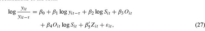
where yit denotes per capita income in country i at time t, Sit is a measure of country size, Oit is a measure of openness, and Zit is a vector of control variables. In this specification, the parameter estimates on openness, country size and their interaction will be our main focus. In the context of the theory presented in Section 2, these variables as well as the Zit variables are to be interpreted as determinants of the steady-state level of per capita income.[364]
3.4.1. Descriptivestatistics
Tables 1-3 display summary statistics for our main variables of interest, averaged over the period 1960-2000. The data on openness, investment rates, growth and income levels, government consumption, and population come from release 6.1 of the Penn World Tables [Heston, Summers and Aten (2002)], which updates their panel of PPP-comparable data to the year 2000. The rest of the data we use in this paper comes from Barro and Lee (1994, subsequently updated to 2000) or from the Central Intelligence Agency (2002). Country size is measured by the log of total GDP or by the log of total population, in order to capture both economic size and demographic size. Throughout, we define trade openness in two ways: as the ratio of imports plus exports in current prices to GDP in current prices, and as the ratio of imports plus exports in exchange rate $U.S. to GDP in PPP $U.S. We label the first variable “nominal openness” and the second one “real openness”.
Recently, Alcala and Ciccone (2003, 2004) have criticized the widespread use of the first measure, have advocated the use of the second, finding that the latter leads to more robust effects of openness on growth. The key difference between the two measure stems from the treatment of non tradable goods. Suppose that trade openness raises productivity, but does so more in the tradable than in the nontradable sector (a plausible assumption). This will lead to a rise in the relative price of nontradables, and a fall in conventionally measured openness under the assumptions that the demand for nontrad-
Table 1
Descriptive statistics (1960-2000 averages)
| Number of observations | Mean | bgcolor=white>Standard deviationMinimum | Maximum | ||
| Average annual growth | 104 | 1.669 | 1.374 | -1.259 | 5.515 |
| Openness ratio (current) | 114 | 64.098 | 41.871 | 14.373 | 322.128 |
| Openness ratio (real) | 114 | 37.363 | 35.376 | 4.350 | 244.631 |
| Log of per capita GDP 1960 | 110 | 7.730 | 0.889 | 5.944 | 9.614 |
| Log of total GDP | 113 | 23.905 | 1.943 | 19.723 | 29.165 |
| Log of population | 114 | 15.763 | 1.678 | 11.019 | 20.670 |
| Fertility rate | 156 | 4.569 | 1.797 | 1.733 | 7.597 |
| Female human capital | 103 | 1.116 | 1.067 | 0.024 | 4.923 |
| Male human capital | 103 | 1.523 | 1.225 | 0.096 | 5.467 |
| Investment rate (% GDP) | 114 | 15.653 | 7.880 | 2.023 | 41.252 |
| Government consumption (% GDP) | 114 | 19.869 | 9.439 | 4.297 | 48.635 |
Table 2
Pairwise correlations for the main variables of interest (1960-2000 averages)
| Average annual growth | Log of total GDP | Log of per capita GDP 1960 | Log of population | Openness ratio (current) | |
| Average annual growth | 1.000 | ||||
| Log of total GDP | 0.338 | 1.000 | |||
| Log of per capita GDP 1960 | 0.172 | 0.436 | 1.000 | ||
| Log of population | 0.125 | 0.853 | -0.058 | 1.000 | |
| Openness ratio (current) | 0.216 | -0.334 | 0.135 | -0.537 | 1.000 |
| Openness ratio (real) | 0.331 | -0.042 | 0.382 | -0.348 | 0.870 |
ables is relatively inelastic, as it may raise the denominator of the conventional measure of openness more than the numerator. So one may observe trade-induced productivity increases going hand in hand with a decline in conventional measures of openness. “Real openness” will address the problem, since the denominator now corrects for international differences in the price of nontradable goods. We show results based on both measures, in order to simultaneously address Alcala and Ciccone’s points and to allow comparability with past results.
Table 2 reveals that both measures of openness are closely related, with a correlation of 0.87. While high, this correlation justifies examining differences in results obtained using each measure. The correlation between our two measures of country size is also high, equal to 0.85. The correlation between openness and country size is negative, whatever the measures of openness and size, and in three out of four cases is of a magnitude between 0.33 and 0.54, confirming past results that small countries are more
Table 3
Conditional correlations (1960-2000)
| Variable | Conditioning statement | Correlation with growth | Number of observations |
| Openness (current) | Log of population > median = 8.807 | 0.104 | 54 |
| Openness (current) | Log of population ≤ median = 8.807 | 0.511 | 50 |
| Openness (current) | Log of GDP > median = 16.700 | 0.301 | 52 |
| Openness (current) | Log of GDP ≤ median = 16.700 | 0.462 | 52 |
| Openness (real) | Log of population > median = 15.715 | 0.131 | 54 |
| Openness (real) | Log of population ≤ median = 15.715 | 0.579 | 50 |
| Openness (real) | Log of GDP > median = 23.607 | 0.223 | 52 |
| Openness (real) | Log of GDP ≤ median = 23.607 | 0.474 | 52 |
| Log of population | Openness (current) > median = 53.897 | 0.107 | 50 |
| Log of population | Openness (current) ≤ median = 53.897 | 0.426 | 54 |
| LogofGDP | Openness (current) > median = 53.897 | 0.324 | 50 |
| LogofGDP | Openness (current) ≤ median = 53.897 | 0.563 | 54 |
| Log of population | Openness (real) >median = 26.025 | -0.089 | 51 |
| Log of population | Openness (real) ≤ median = 26.025 | 0.587 | 53 |
| Log of GDP | Openness (real) > median = 26.025 | 0.137 | 51 |
| Log of GDP | Openness (real) ≤ median = 26.025 | 0.625 | 53 |
Notes. Medians computed from individual samples, while correlations are common sample correlations. Growth: average annual growth, 1960-2000.
open, and suggesting that an omission of openness in a regression of growth on country size would understate the effect of size. Finally, while the simple correlation between growth and size is 0.33 when size is measured by the log of total GDP, and the correlation between openness and growth is equal to 0.21 or 0.33 (when openness is measured in current or “real terms”, respectively).
Preliminary evidence on Propositions 1 and 2 can be gleaned from conditional correlations displayed in Table 3. This table presents correlations of openness and growth conditional on country size being greater or lower than the sample median, and correlations of country size and growth conditional on openness being greater or lower than the sample median. For the sake of illustration, let us focus on the log of population as a measure of size and on current openness as a measure of openness (the results are qualitatively unchanged when using the other measures). The correlation between openness and growth is 0.51 for small countries (those smaller than 6.7 million inhabitants), and only 0.10 for large countries. Similarly, the correlation between country size and growth is 0.11 for open countries, and 0.43 for closed ones. This provides suggestive evidence that openness and country size are substitutes, and that the correlation between size and growth falls with the level of openness. To fully evaluate this claim, we now turn to panel data growth regressions.
3.4.2. Growth, openness and size: panel regressions
Tables 4-6 present Seemingly Unrelated Regression (SUR) estimates of regressions of growth on openness, country size and their interaction, as well as additional controls. The SUR estimator amounts to a flexible form of the random-effects panel estimator, which allows for different covariances of the error term across time periods.[365] Its use
Table 4
Constrained SUR estimates (size = log of population, openness = current openness)
| (1) | (2) | (3) | (4) | |
| Size * Openness (current) | -0.006** | -0.006** | -0.007** | -0.005* |
| (0.002) | (0.002) | (0.002) | (0.002) | |
| Size | 0.493** | 0.481** | 0.326* | 0.412** |
| (0.123) | (0.120) | (0.153) | (0.138) | |
| Openness (current) | 0.057** | 0.055** | 0.059** | 0.054** |
| (0.015) | (0.014) | (0.020) | (0.018) | |
| Log of initial per capita income | - | 0.185 (0.112) | -1.157** (0.248) | -1.109** (0.230) |
| Fertility | - | - | -0.332** (0.118) | -0.479** (0.110) |
| Male human capital | - | - | 0.090 (0.279) | 0.337 (0.253) |
| Female human capital | - | - | -0.139 (0.327) | -0.260 (0.299) |
| Government consumption (% GDP) | - | - | -0.052** (0.013) | -0.035** (0.012) |
| Investment rate (% GDP) | - | - | 0.133** (0.016) | 0.090** (0.016) |
| Intercept | -3.274** | -4.600** | 8.530** | 8.840** |
| (1.175) | (1.355) | (3.085) | (2.84) | |
| Intercept, 1970-1979 | - | - | - | 8.170** (2.87) |
| Intercept, 1980-1989 | - | - | - | 7.030* (2.86) |
| Intercept, 1990-2000 | - | - | - | 6.960* (2.81) |
| Number of countries (periods) | 104 (4) | 104 (4) | 80 (4) | 80 (4) |
| Adjusted TNsquared | 0.15 0.01 | 0.15 0.02 | 0.12 0.22 | 0.38 0.23 |
| 0.11 0.03 | 0.10 0.05 | 0.35 0.14 | 0.47 0.23 |
Notes. Standard errors in parentheses.
* significant at 5% level; **significant at 1% level.
Table 5
Constrained SUR estimates (size = log of GDP, openness = current openness)
| (1) | (2) | (3) | (4) | |
| Size * Openness (current) | -0.005** | -0.005** | -0.003t | -0.003t |
| (0.001) | (0.001) | (0.002) | (0.002) | |
| Size | 0.532** | 0.592** | 0.325* | 0.438** |
| (0.099) | (0.113) | (0.139) | (0.125) | |
| Openness (current) | 0.089** | 0.093** | 0.064* | 0.063* |
| (0.024) | (0.025) | (0.030) | (0.027) | |
| Log of initial per capita income | - | -0.171 | -1.252** | -1.342** |
| (0.143) | (0.247) | (0.230) | ||
| Fertility | - | - | -0.317** | -0.466** |
| (0.119) | (0.109) | |||
| Male human capital | - | - | -0.011 | 0.268 |
| (0.282) | (0.254) | |||
| Female human capital | - | - | -0.045 | -0.184 |
| (0.331) | (0.300) | |||
| Government consumption (% GDP) | - | - | -0.050** | -0.034** |
| (0.013) | (0.012) | |||
| Investment rate (% GDP) | - | - | 0.126** | 0.081** |
| (0.017) | (0.016) | |||
| Intercept | -8.163** | -7.937** | 6.358 | 6.740* |
| (1.758) | (1.804) | (3.471) | (3.13) | |
| Intercept, 1970-1979 | - | - | - | 6.010 |
| (3.16) | ||||
| Intercept, 1980-1989 | - | - | - | 4.820 |
| (3.16) | ||||
| Intercept, 1990-2000 | - | - | - | 4.680 |
| (3.12) | ||||
| Number of countries (periods) | 104 (4) | 104 (4) | 80 (4) | 80 (4) |
| Adjusted TNsquared | 0.11 0.01 | 0.12 0.01 | 0.13 0.22 | 0.41 0.24 |
| 0.09 0.02 | 0.07 0.02 | 0.35 0.06 | 0.47 0.19 |
Notes. Standard errors in parentheses.
tsignificant at 10% level;
* significant at 5% level;
**significant at 1% level.
in cross-country work is now widespread [see, for example, Barro and Sala-i-Martin (1995)]. The panel consists of four periods of 10 year-averages (1960-1969, 19701979, 1980-1989 and 1990-1999), and up to 113 countries. The estimation procedure is to formulate one equation per decade, constrain the coefficients to equality across periods, and run SUR on the resulting system of equations.[366]
Table 6
Constrained SUR estimates (using real openness)
| Size = log of population | Size = log of GDP | |||
| (1) | (2) | (3) | (4) | |
| Size * Real openness | -0.004* | -0.006˛ | -0.008** | -0.007* |
| (0.002) | (0.003) | (0.002) | (0.003) | |
| Size | 0.250** | 0.229˛ | 0.496** | 0.424** |
| (0.093) | (0.129) | (0.096) | (0.126) | |
| Real openness | 0.075* | 0.094˛ | 0.198** | 0.185** |
| (0.031) | (0.052) | (0.050) | (0.068) | |
| Log of per capita income, 1960 | 0.092 | -1.295** | -0.244 | -1.489** |
| (0.135) | (0.235) | (0.160) | (0.238) | |
| Fertility | — | -0.552** | — | -0.537** |
| (0.111) | (0.110) | |||
| Male human capital | — | 0.247 | — | 0.205 |
| (0.259) | (0.254) | |||
| Female human capital | — | -0.162 | — | -0.130 |
| (0.298) | (0.292) | |||
| Government consumption (% GDP) | — | -0.033** | — | -0.033** |
| (0.012) | (0.012) | |||
| Investment (% GDP) | — | 0.090** | — | 0.076** |
| (0.016) | (0.017) | |||
| Intercept | -3.318 | — | -8.823** | — |
| (1.733) | (2.091) | |||
| Number of countries (periods) | 104 (4) | 80 (4) | 104 (4) | 80 (4) |
| Adjusted R-squared | -0.18 -0.01 | 0.33 0.21 | -0.14 0.03 | 0.35 0.19 |
| -0.07 0.02 | 0.47 0.22 | -0.03 0.06 | 0.50 0.24 | |
Notes. Standard errors in parentheses.
^significant at 10% level;
* significant at 5% level; **significant at 1% level.
Columns (2) and (4) estimated with period specific intercepts (time effects not reported). Other specifications available upon request.
Table 4 present estimation results when the measure of country size is the log of population and the measure of openness involves variables in current prices. In all specifications, the parameter estimates on our three variables of interest (openness, country size and their interaction) are of the predicted sign and all are significant at the 5% level (and often at the 1% level). This holds whether we enter these variables alone [column (1)], whether we control for initial income [column (2)], whether we control for a long list of common growth regressors [column (3)] and whether we include time specific effects in addition to all the controls [column (4)]. Moreover, Table 5 shows that the results change little when size is measured by the log of total GDP, although the level of significance is reduced somewhat in the specifications that include many control variables. Finally, Table 6 shows that using “real openness” does not modify the overall pattern of coefficients. In fact our results are generally stronger (in the sense of the estimated coefficients being larger in magnitude) when using this measure of openness. Similar estimates in Alcala and Ciccone (2003, written after first draft of this paper) lend further support to our results. They show how controlling for a host of additional variables including institutional quality does not change the nature of these results and that the use of “real openness” leads to coefficients that are larger and more robust than when using “nominal openness”.
3.5. Endogeneity of openness: 3SLS estimates
Openness, especially when defined as the volume of trade divided by GDP (however deflated), may be an endogenous variable in growth regressions. As described above, in an important paper Frankel and Romer (1999) have developed a innovative instrument to deal with potential endogeneity bias in growth and income level regressions. We use our own set of geographic variables as well as Frankel and Romer’s instrument to address potential endogeneity. Our panel data IV estimator relies on a three stage least squares (3SLS) procedure. This estimator achieves consistency through instrumentation, and efficiency through the estimation of cross-period error covariance terms. Table 7 presents parameter estimates of our basic specification when the list of instruments includes geographic variables, namely dummy variables for small countries, islands, small islands, landlocked countries and the interaction term between each of these measures and country size.[367] Again, the results are consistent with previous observations, namely the pattern of coefficients suggested by theory is maintained. In the specification with all the controls, the statistical significance of the coefficients of interest is reduced slightly when real openness is used instead of current openness (Table 8), though all remain significant at the 10% level. The signs of the main coefficients of interest are maintained and the magnitude of the openness coefficient is raised in all specifications, confirming the results of Alcala and Ciccone (2003, 2004).[368]
Finally, Table 11 shows the same results using the geography-based instrument from Frankel and Romer (1999), as well as the interaction term between this variable and country size. In all specifications, the signs and basic magnitudes of the coefficients of interest are unchanged (although when openness is entered in “real” terms, the estimates cease to be statistically significant at the 5% level). Spolaore and Wacziarg (2005)
Table 7
Constrained 3SLS estimates (current openness)
| Size = log of population | Size = log of GDP | |||||
| (1) | (2) | (3) | (4) | (5) | (6) | |
| Size * Openness (current) | -0.008** | -0.007** | -0.008** | -0.007** | -0.010** | -0.003^ |
| (0.002) | (0.002) | (0.003) | (0.002) | (0.002) | (0.002) | |
| Size | 0.507** | 0.634** | 0.375* | 0.677** | 1.070** | 0.314* |
| (0.157) | (0.144) | (0.176) | (0.143) | (0.167) | (0.158) | |
| Openness (current) | 0.068** | 0.073** | 0.069** | 0.129** | 0.193** | 0.060^ |
| (0.020) | (0.018) | (0.024) | (0.038) | (0.039) | (0.036) | |
| Log of initial per capita income | - | 0.147 | -1.157** | — | -0.525** | -1.257** |
| (0.117) | (0.251) | (0.167) | (0.247) | |||
| Fertility | — | — | -0.330** | — | — | -0.319** |
| (0.120) | (0.121) | |||||
| Male human capital | - | — | 0.125 | — | — | -0.017 |
| (0.281) | (0.283) | |||||
| Female human capital | — | — | -0.171 | — | — | -0.039 |
| (0.329) | (0.332) | |||||
| Government consumption (% GDP) | — | — | -0.052** | — | — | -0.050** |
| (0.013) | (0.013) | |||||
| Investment rate (% GDP) | — | — | 0.134** | — | — | 0.126** |
| (0.016) | (0.017) | |||||
| Intercept | -2.701 | -5.945** | 8.178* | -10.843** - | 14.269** | 6.596 |
| (1.537) | (1.513) | (3.299) | (2.604) | (2.561) | (3.813) | |
| Number of countries (periods) | 104 (4) | 104 (4) | 80 (4) | 104 (4) | 104 (4) | 80 (4) |
| Adjusted TNsquared | 0.13 0.05 | 0.18 0.02 | 0.13 0.21 | 0.12 0.07 | 0.25 0.02 | 0.28 0.35 |
| 0.19 0.01 | 0.11 0.03 | 0.34 0.15 | 0.13 0.01 | 0.16 0.24 | 0.140.18 | |
Notes. Standard errors in parentheses.
^significant at 10% level;
* significant at 5% level;
**significant at 1% level.
Instruments used: dummies for small country, island, small island, landlocked country and the interaction of each of these measures with the log of country size.
present more evidence on this type of regression, by treating estimating a simultaneous equations system for the endogenous determination of openness and growth jointly. Their results are similar in spirit to those presented here.
Alcala and Ciccone (2003) present further results along the same lines, and also explicitly consider institutional quality variables in addition to performing further sensitivity tests. Their empirical results are very consistent with ours, suggesting that predictions on the relationship between trade, country size and growth implied by our model are confirmed when the “real” measure of openness is used instead of nominal openness.
Table 8
Constrained 3SLS estimates (real openness)
| Size = log of population | Size = log of GDP | |||||
| (1) | (2) | (3) | (4) | (5) | (6) | |
| Size * Real openness | -0.006* | -0.006* | -0.007˛ | -0.014** | -0.014** | -0.007* |
| (0.003) | (0.003) | (0.004) | (0.003) | (0.003) | (0.003) | |
| Size | 0.280** | 0.317** | 0.248˛ | 0.630** | 0.768** | 0.440** |
| (0.107) | (0.103) | (0.146) | (0.111) | (0.124) | (0.141) | |
| Real openness | 0.100* | 0.098* | 0.1111 | 0.350** | 0.361** | 0.195* |
| (0.040) | (0.038) | (0.062) | (0.073) | (0.071) | (0.079) | |
| Log of per capita | - | 0.017 | -1.277** | - | -0.526** | -1.493** |
| income, 1960 | (0.157) | (0.237) | (0.187) | (0.239) | ||
| Fertility | — | - | -0.543** | - | - | -0.536** |
| (0.112) | (0.110) | |||||
| Male human capital | - | - | 0.269 | - | - | 0.206 |
| (0.260) | (0.255) | |||||
| Female human capital | - | - | -0.167 | - | - | -0.13 |
| (0.299) | (0.292) | |||||
| Government | - | - | -0.033** | - | - | -0.033** |
| consumption (% GDP) | (0.012) | (0.012) | ||||
| Investment (% GDP) | - | - | 0.092** | - | - | 0.075** |
| (0.017) | (0.017) | |||||
| Intercept | -2.941 | -3.922* | - | -13.883** | -13.503** | - |
| (1.706) | (1.919) | (2.721) | (2.679) | |||
| Number of | 104 (4) | 104 (4) | 80 (4) | 104 (4) | 104 (4) | 80 (4) |
| countries (periods) | ||||||
| Adjusted R-squared | -0.17 -0.01 | -0.20 -0.01 | 0.33 0.22 | -0.10 0.02 | -0.21 -0.01 | 0.35 0.19 |
| -0.09 0.01 | -0.06 0.00 | 0.46 0.22 | -0.15 -0.01 | -0.08 -0.02 | 0.50 0.24 | |
Notes. Standard errors in parentheses.
^significant at 10% level;
* significant at 5% level;
**significant at 1% level.
Instruments used: dummies for small country, island, small island, landlocked country, and the interaction of each of these measures with the log of population.
Columns (3) and (6) estimated with period specific intercepts (time effects not reported). Other specifications available upon request.
3.5.1. Magnitudesandsummary
While the pattern of signs and the statistical significance of the estimates presented above is consistent with our theory, the effects could still be small in magnitude. However, they are not. To illustrate the extent of the substitutability between country size and openness, let us choose a baseline regression. Consider column (4) of Table 4 - this involves using the log of population as a measure of size, current openness as a
Table 9
First-stage F-tests for the instruments (current openness)
| Specification | Endogenous variable | Openness (current) | Openness * Size |
| Size = log of population | |||
| 1 | F-statistics p value | 4.83 | 3.92 |
| 0.00 | 0.00 | ||
| 2 | F-statistics p value | 5.63 | 6.28 |
| 0.00 | 0.00 | ||
| 3 | F-statistics p value | 4.22 | 4.49 |
0.00 0.00
Size = log ofGDP
| 4 | F -statistics p value | 5.61 | 6.25 |
| 0.00 | 0.00 | ||
| 5 | F -statistics p value | 10.38 | 11.23 |
| 0.00 | 0.00 | ||
| 6 | F -statistics p value | 7.52 | 7.34 |
| 0.00 | 0.00 |
Note. F-tests on the instruments from a regression of each endogenous variable on the list of instruments plus the exogenous regressors in each specification.
Table 10
First-stage F -tests for the instruments (real openness)
| Specification | Endogenous variable | Openness (constant) | Openness * Size |
| Size = | log of GDP | ||
| 1 | F -statistics p value | 4.45 | 4.95 |
| 0.00 | 0.00 | ||
| 2 | F -statistics p value | 9.09 | 9.92 |
| 0.00 | 0.00 | ||
| 3 | F -statistics p value | 10.75 | 10.80 |
0.00 0.00
Size = log of population
| 4 | F -statistics p value | 4.55 | 3.52 |
| 0.00 | 0.00 | ||
| 5 | F -statistics p value | 6.25 | 7.18 |
| 0.00 | 0.00 | ||
| 6 | F -statistics p value | 5.67 | 7.20 |
| 0.00 | 0.00 |
Note. F-tests on the instruments from a regression of each endogenous variable on the list of instruments plus the exogenous regressors in each specification.
measure of openness, and a wide range of controls in the growth regression. Consider a country with the median size. In our sample, when the data on log population are
Table 11
Constrained 3SLS estimates (using Frankel and Romer’s instrument)
| Size = log of population | Size = log of GDP | |||
| Current openness (1) | Real openness (2) | Current openness Real openness | ||
| (3) | (4) | |||
| Size * Openness | -0.008** | -0.010˛ | -0.003˛ | -0.009* |
| (0.003) | (0.006) | (0.002) | (0.004) | |
| Size | 0.435* | 0.273 | 0.399* | 0.452** |
| (0.180) | (0.197) | (0.166) | (0.173) | |
| Openness | 0.128** | 0.163? | 0.089˛ | 0.242* |
| (0.041) | (0.088) | (0.049) | (0.099) | |
| Log of initial per capita income | -1.114** | -1.254** | -1.282** | -1.433** |
| (0.251) | (0.252) | (0.245) | (0.255) | |
| Fertility | -0.307* | -0.354** | -0.290* | -0.348** |
| (0.122) | (0.120) | (0.125) | (0.118) | |
| Male human capital | 0.105 | -0.011 | -0.036 | -0.086 |
| (0.280) | (0.291) | (0.283) | (0.284) | |
| Female human capital | -0.164 | -0.023 | -0.043 | 0.031 |
| (0.321) | (0.327) | (0.325) | (0.320) | |
| Government consumption (% GDP) | -0.053** | -0.052** | -0.051** | -0.052** |
| (0.013) | (0.013) | (0.013) | (0.013) | |
| 0.131** | 0.130** | 0.122** | 0.112** | |
| (0.017) | (0.017) | (0.017) | (0.019) | |
| Intercept | 3.959 | 7.991 | 2.219 | 2.694 |
| (4.408) | (4.296) | (4.948) | (4.547) | |
| Number of countries (periods) | 80 (4) | 78 (4) | 80 (4) | 80 (4) |
| Adjusted R-squared | 0.12 0.21 | 0.04 0.20 | 0.11 0.23 | 0.02 0.18 |
| 0.36 0.14 | 0.37 0.10 | 0.37 0.02 | 0.40 0.12 | |
Notes. Standard errors in parentheses.
^significant at 10% level;
* significant at 5% level;
**significant at 1% level.
Instruments used: Frankel-Romer instrument for openness and its interaction with the log of GDP.
averaged over the period 1960-2000, the median country turns out to be Mali (where the log of population is 8.802 - this corresponds to an average population of 6.6 million over the sample period). The effect of a one standard deviation change in openness (a change of 42 percentage points) on Mali’s annual growth is estimated to be 0.419 percentage points. In contrast, in the smallest country in our sample (the Seychelles), the same change in openness would translate into an increase in growth of 1.40 percentage points. The effect of a marginal increase in openness on growth becomes zero when the log of population is equal to 10.8, which is the size of France (in our sample, only 13 countries are larger).
Conversely, the effect of size at the median level of openness, which is attained by South Korea (with a trade to GDP ratio of 54% on average between 1960 and 1999), the effect of multiplying the country’s size by 10 would be to raise annual growth by 0.33 percentage points. In contrast, a relatively closed country such as Argentina (with a trade to GDP ratio of 15% on average between 1960 and 1998) would experience an increase in growth of 0.78 percentage points from decoupling its population. The effect of size on growth attains zero when openness reaches 82.4% (in our sample, 26 countries had a higher level of average openness over the 1960-1999 period). Using the results obtained with “real” measures of openness the magnitude of our results would typically be even larger.
Whether one “believes” these actual magnitudes or not, the signs and statistical significance of our variables of interest are very robust features of the data and independently confirmed and reinforced by Alcala and Ciccone (2003). When evaluating the effects of scale on growth, it is essential to view scale as attainable either through a large domestic market, or through trade openness. Ignoring either would lead to underestimating scale effects in income. This section and the literature from which it is inspired has sought to bring together the research on the impact of trade on growth and the research on the impact of economic scale on growth, and in doing so has empirically established a substitutability between openness and country size.
4.