Policy

It is worth pausing at this point and noting that the mechanism generating a currency crisis in this chapter departs from most exist­ing models of currency crises, as it relies entirely upon private

110 The Third Generation Approach to Currency Crises sector behavior.

This does not imply that our approach of currency crises cannot be linked to previous theories: as we shall try to argue in this section, it complements previous explanations, for example, by Krugman (1979) or Obstfeld (1994). In Subsection 5.3.1, we analyze an explicitly fixed exchange rate regime, while in Subsection 5.3.2 we briefly consider the government's balance sheet constraint and its interaction with private firms.

5.3.1 Exchange rates regimes

To illustrate the fact that the specific exchange rate regime is not the most crucial element in the analysis, we now consider the case of an economy with an (initially) fixed exchange rate system. While such a system can maintain a stable exchange rate when the eco­nomy is hit by small shocks, the initial exchange rate regime has little influence in preventing a currency crisis following a large shock.

In a fixed exchange rate system, the role of the central bank's international reserves, as well as the rule leading to the abandon­ment of the fixed rate, need to be specified. Fixing the exchange rate in our model implies a given path of money supply in all periods t > 1, possibly through the use of international reserves; furthermore, it implies that at date t = 1, the central bank can no longer use the interest rate i₁ as a policy instrument, if the interest parity condition is to hold perfectly.^[35] More formally, assume that the exchange rate is initially fixed at E_t = E.

equation (5.2) in period 2 can be rewritten as:

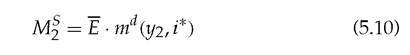
where money supply M2f is now endogenous. On the other hand, equilibrium of the central bank's balance sheet imposes the condition :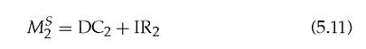

where DC2 is domestic credit, typically claims on the government, and IR₂ represents international reserves expressed in domestic currency in period 2.

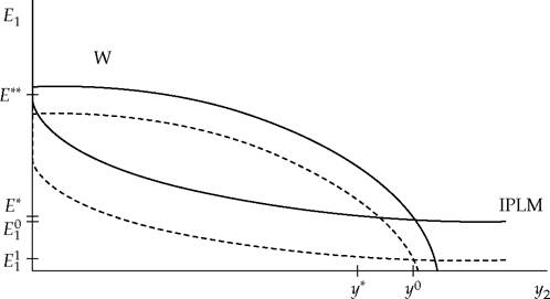
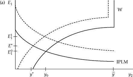
To understand why a large real shock may force a government to abandon the fixed exchange rate regime and can precipitate the occurrence of a currency crisis, assume that international reserves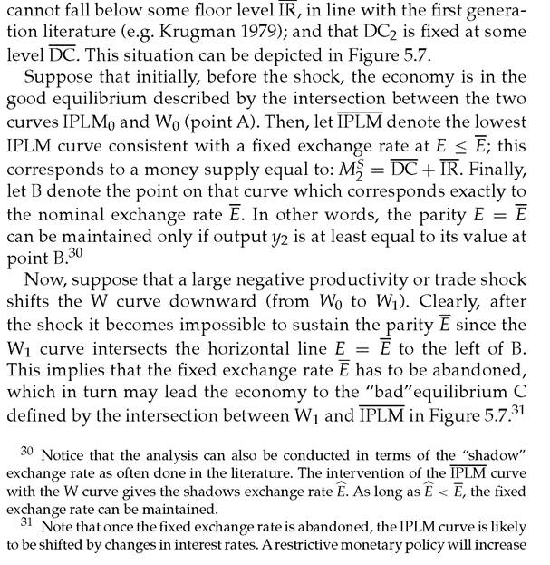

Fig. 5.7 A large real shock may trigger a currency crisis in a fixed exchange rate system.

Source: Aghion et al. (2001), figure 6.

It is important to note that the decline in reserves that triggers the currency crisis is caused here by the underlying weakness in the financial health of private firms and not by a fiscal deficit as in the first generation models of currency crises. This does not mean that government behavior and public deficits cannot also have an effect on the occurrence of currency crises, as we will argue in the next subsection. Thus, the potential sources of cur­rency crises highlighted in first generation models, can also be

i1 and shift IPLM down. However, the IPLM may still shift up thereafter due to an increase in i2, which itself is caused by the expectation of a further depreciation (as in Krugman 1979).

The Third Generation Approach to Currency Crises 113 shown to be relevant when analyzed in the context of the “third generation"model in this chapter.

Similarly, we can use our framework to analyze credibility aspects of the kind emphasized by the second generation of currency crises models. For example, instead of assuming a floor level of international reserves, suppose that the government's objective is to minimize a loss function which increases both with the size of output declines and the extent of a currency devaluation. Then, if output depends negatively on the nominal interest rate as will be discussed in Section 5.4, we can easily re-obtain the multiple equilibrium result of the second generation models.^[36] To see this, note first that an increase in the high interest rate i0 reduces output y2 and therefore increases the likelihood of a currency depreciation in period 1. Thus, if at date 0 investors increase their expectation of a currency devaluation in period 1, the interest parity condi­tion in period 0 implies that i0 must increase, but this in turn will cause an output fall, thereby making the expectation of a currency depreciation self-fulfilling.

Two conclusions can be drawn from these illustrations. First, our model also explains currency crises in economies with an ini­tially fixed exchange rate. Second, first- and second generation features can interact with the balance sheets of private firms and thereby lead to a currency crisis through the same basic mechanism as above.

What does our model tell us about the optimal exchange rate regime? In the case of large shocks, we have just argued that the outcome is likely to be quite similar under a fixed or a floating exchange rate regime. However, this conclusion would change if a government could credibly commit to never abandon a given exchange rate parity, for example by instituting a currency board or some kind of dollarization policy. Nevertheless, these strategies are not without risks. One potential drawback of maintaining a fixed exchange rate regime over a long period, for example, through establishing a currency board, is the fact that combined with persistent price rigidity it can lead to currency overvaluation (i.e.

5.3.2 Public versus private debt in currency crises

In the first generation of currency crises models, it is the incon­sistency between public sector behavior and a fixed exchange rate that is at the source of a crisis. In this subsection, we emphas­ize the interaction between fiscal variables and the private sector. This interaction can take two forms. First, a fiscal shock such as an increase in government expenditure or a decline in tax revenues, may crowd out the private sector and thereby lead to a currency crisis. Second, a negative shock to fundamentals or to expecta­tions may affect both the private and the public sector in such a way that the deterioration of the private sector's financial health is exacerbated by the deterioration of the public budget.

To organize thoughts it is useful to look at a consolidated gov­ernment's balance sheet. Assume that government activities are

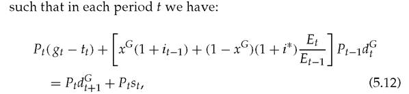
where g_t and t_t denote real expenditure and revenue; dG is the privately held public debt contracted in period t - 1 and due to be reimbursed in period t; x^G denotes the fraction of government debt which is in domestic currency; and st represents real seigniorage revenue.

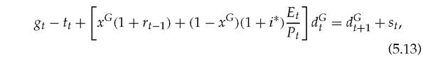
The first important point that emerges from equation (5.13) is that public sector's debt is affected negatively by unanticip­ated currency depreciations in exactly the same way as private sector's debt.^[39] Thus, it is not difficult to imagine a “second generation"model (e.g. in the line of Obstfeld 1994) where mul­tiple equilibria and the possibility of currency crises, stem from a high proportion of public foreign currency debt. This is in sharp contrast with the existing literature (again, see Obstfeld 1994) where currency crises occur in economies with high pro­portions of domestic currency debt and where having foreign currency debt can help avoid a crisis altogether. Behind this con­trast lies the fact that previous models would typically assume ex post PPP and no foreign price uncertainty, which implies that foreign currency bonds are a perfect hedge against currency fluc­tuations. The experience with countries issuing foreign currency

116 The Third Generation Approach to Currency Crises debt, such as Mexico with its dollar-linked tesobonos, tends to sup­port the view that public foreign currency debt is not always a stabilizing influence.

Let us now turn to the interaction between the private and the public sector. Consider for example an increase in the primary fiscal deficit at time one, g1 — f₁.3⁶ The impact on the private sector depends on which other variable adjusts in (5.13). First, assume that an increase in the deficit is financed by an increase in seigniorage s1. This implies an increase in money growth from period 2 on, which in particular means an increase in M^s and in ⅛ (due to an increase in π3).

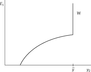
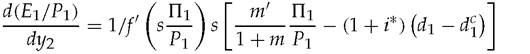
Now, suppose that the increased budget deficit leads to a reduc­tion in the amount of lending to firms, through a decline in the credit-multiplier μ. This may be due to some standard crowding out between public and private debt; or because a larger deficit would reduce the amount of government funds available to save insolvent or illiquid banks or firms from bankruptcy.^{[40] [41] This decline in μ will lead to a downward shift of the W curve, which again may result in the possibility of a crisis. Here again, a negative shock on the public sector leads to a crisis through its impact on private firms.}

To summarize our discussion in this section, we have argued that although a currency crisis may be directly triggered by a weaken­ing of private sector firms' balance sheets, it can also be provoked by imbalances in the public sector. This may help explain crises episodes like Brazil in the late 1990s, where the corporate and banking sectors suffered from the increasing fiscal imbalances.

5.3.3 Monetarypolicy

The appropriate monetary policy response to the recent crises has been a hotly debated issue. Our model, being an explicitly mon­etary model, is well suited as a framework for discussing these issues.^[42] Consider the model developed in Sections 5.1 and 5.2. Suppose it is known that the economy has a significant chance of switching to the currency crisis equilibrium, either because of a shift in expectations or because of a real shock. In other words, we are now in a situation such as the one depicted in Figure 5.5(c). Can the monetary authorities do anything that would guarantee that the economy avoids a currency crisis?

Obviously what they need to do is to shift the IPLM curve so that the economy moves to a configuration of the type shown in Figure 5.5(a). Figure 5.8 shows this case. The correct policy response in this case is obviously to increase the interest rate i1 and/or decrease MS so that the IPLM curve shifts downward.

Fig. 5.8 Currency crisis can be avoided by using tight monetary policy. Source: Aghion et al. (2001), figure 7.

Figure 5.8 thus shows a situation in which the currency crisis can be avoided and initial output be restored, through appreciating the currency to Ep This can be seen as the standard case for a tight monetary policy during a currency crisis.

The main argument of those defending a lax monetary policy, however, is that interest rate increases negatively affect output. To take this into consideration, we consider a model of the credit mar­ket, developed in the Appendix, where credit depends negatively on the real interest rate, that is, m(r_t) with m' < 0. To see how this additional effect modifies the W curve we have to take account of the relationship between the real interest rate and the exchange rate. Using the interest parity condition and the definition of the real interest rate, we have: 1 + r1 = (1 + i*)P1∕E1. This allows us to rewrite the credit multiplier as m_t = m(E1∕P1), where m' > 0.39 Equation (5.5) then gets re-expressed in the form:

Changes in E1 (with P1 fixed) have now two effects on y2. In addi­tion to an increase in the foreign currency debt burden of domestic entrepreneurs, an increase in E1 reduces the real interest rate r1, which in turn relaxes the credit constraint and therefore increases the availability of funds d₂ at the beginning of period 2. The slope of the W curve depends on the relative importance of the two effects. Figure 5.4, with μ constant, represents the case where the foreign currency debt effect dominates. In Figure 5.9 the relation­ship between y2 and E1 is positive. It becomes a vertical line at ó when μ is so large (r1 so small) that the credit constraint is no longer binding. Note that other shapes of the W curve are possible. In particular, it might be positively sloped for low values of E₁ and negatively sloped for high values of E1.

39 The m function is increasing in E1/P1, since a high value of E1/P1 predicts that future inflation will be high relative to future depreciation, and therefore depresses the real interest rate.

Fig. 5.9 The slope of the W curve if credit constraint effect dominates. Source: Aghion et al. (2001), figure 8.

The exact expression for the slope of the W curve (from equation (5.14) is:

where s = (1 — α)(1 + m). It is clear from this expression that when there is no foreign currency debt, that is, when = d1, the W curve is always upward-sloping. As the proportion of foreign currency debt increases, the slope of the W curve increases, turning negative; the limit is achieved at d^c₁ = 0. When credit markets are completely absent, that is, when m = 0, we must have d^c₁ = d₁ = 0 and therefore the W curve would always be vertical. This is as it should be: when there is no credit, exchange rate variations should not affect investment capacity. The W curve is also vertical when m is very large and therefore the credit constraint is not binding: in this case output should not be affected by the profitability of the firm sector. In the intermediate case where there is a substantial amount of borrowing but the credit constraint still binds, the W curve can be downward-sloping and relatively flat.^[43] This turns out to be the case where we can have currency crises. In that sense currency crises will be associated with countries that are at an intermediate level of financial development.

Let us now examine monetary policy where the W curve slopes up as in Figure 5.10(a). In this case, consider a negative shock that

Fig. 5.10 Monetary policy where the W curve (a) slopes up, (b) has both a positive and a negative slope.

Source: Aghion et al. (2001), figure 9.

The Third Generation Approach to Currency Crises 121 has reduced output from y⁰ to y* and caused a currency depre­ciation from E0 to E*. Then, an expansionary monetary policy, that is, a decrease in i1 or an increase in M%, can help us main­tain the initial level of output, y⁰, though such policy will shift the IPLM curve upward and therefore induce a further currency depreciation to Ep Notice, however, that there is no crisis, either potential or actual, in this case. The case where the W curve slopes down is the same as the one analyzed in Figure 5.8, so that an interest rate increase can avoid a currency crisis. Finally, there may still be more complex situations where the W curve has both a positive and a negative slope, as in Figure 5.10(b). In that case a leftward shift in the W curve following a negative shock may again lead to multiple equilibria and a potential crisis. While the optimal monetary policy is now restrictive it can only eliminate the risk of a currency crisis at the cost of reducing aggregate output down to y].

To summarize, as in the extended model with competitiveness effects, an expansionary policy can be justified only in situations where the Wcurve is upward-sloping, that is, only if currency crises are impossible. The intuition behind this claim is as follows: the effect of lowering nominal interest rates can be beneficial in this model only if lowering nominal interest rates also lowers real interest rates, which in turn raises μ and has an expansionary effect on output.^[44] Now, the only way to lower real interest rates in our model, is to allow the currency to slide down so that the expec­ted future appreciation of the domestic currency can compensate bond holders for the lower interest rate. But allowing the currency to slide in a crisis-prone economy will cause output to contract (this is precisely what makes the economy crisis prone) and this output contraction in turn will lead to further depreciation of the local currency and push the economy closer to a crisis. There­fore a currency crisis in our model demands a tight monetary policy.^[45]

5.4