The occurrence of currency crises

In this section we focus on the first two periods of production and lending t = 1,2, so that we can analyze the mechanics of the model using simple graphical representation. In particular, we describe the mechanism leading to multiple expectational equilibria and the subsequent possibility of a currency crisis.

5.2.1 A graphical representation of the model

Throughout the remaining part of the chapter, we concentrate on the case where the nominal interest rate in period 2, ⅛, is main­tained constant by monetary policy in subsequent periods.²⁰ In other words, we implicitly assume that the government follows an interest rate targeting or inflation rate targeting (π3 is fixed) policy.²¹ In Aghion et al. (2004b), we show that this assumption can be relaxed without significantly altering the results.²² Taking ⅛ as given, the mechanics of the model will now be shown to be fully described by two curves in the (Ei,y2) space: an IPLM ("Interest-Parity-LM")

²⁰ Jeanne (2000b) presents first- and second generation models using a related two-period approach.

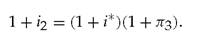
²¹ Indeed, as shown above, we have:

²² For example, suppose that the government targets the rate of money growth z instead, and for simplicity let us take the inflation rate in period 4, π4, as given; then using the fact that:

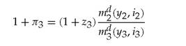
and:

we can endogeneize /'2 as a function of y2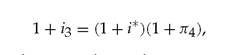and y3, increasing in y2 and decreasing in y₃. In particular, by decreasing y₃, a tight monetary policy, that is, an increase in the nominal interest rate i1, in period 1, will induce an increase in i2.

The IPLM curve is completely standard: it is simply obtained by combining the IP condition (5.1) with the LM equation (5.2) at t = 2 (i.e. LM2) in which the period-2 nominal interest rate ⅛ is taken as given. Using the PPP assumption P2 = E^e₂ = E2 (the latter equality follows from the absence of shock in period 2) we get:

MS m^d (y2, i2)'

which provides a negative relationship between E1 and y2. This relationship is shown in Figure 5.3 as the IPLM curve.^[31] It is easy to see why the IPLM curve slopes down: an increase in (expec­ted) future output y₂ increases the demand for money (i.e. for domestic currency) in period 2, which in turn will naturally gen­erate a nominal currency appreciation in that period, that is, a

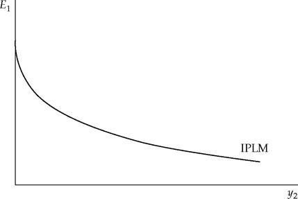
Fig. 5.3 IPLM curve.

Source: Aghion et al. (2001), figure 2.

104 The Third Generation Approach to Currency Crises reduction in E2 = P2. The anticipation of a currency appreciation "tomorrow"(i.e. in period 2) increases the attractiveness of hold­ing domestic currency today, and therefore induces a currency appreciation today, that is, a reduction in E1.

The IPLM curve can be shifted by changes in monetary policy at date t = 1, 2. For example, a tight monetary policy which reduces M⁵ or increases ⅛ (from 5.4), results in a nominal currency appre­ciation, that is, a reduction in E1 for any given y2.

The slope of the IPLM curve also depends on how mobile capital is and the extent of substitutability between domestic and foreign currency assets. We have so far assumed perfect mobility and per­fect substitutability. Relaxing the first assumption, for example, by introducing the possibility of capital controls, will weaken the relationship between i1 and E1. In the extreme case of no capital mobility, the IPLM curve disappears. Relaxing the second assump­tion introduces a foreign exchange risk premium, a case which is examined at the end of Section 5.2.2. In that case what matters are the factors that determine the premium, such as transaction costs and market thinness.

While the IPLM curve is directly drawn from standard macro­economic textbooks and holds even when credit markets are perfect, the W curve captures the effect of imperfect credit markets. It is given by equation (5.5):

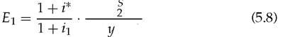
At the beginning of period 1, all variables on the right-hand side of (5.9) are fixed except for E1 (P1 is given since prices are preset and fixed for the entire period 1).^[32] Changes in E1(with P1 fixed) have a negative effect on y2: an increase in E1 (a depreciation)

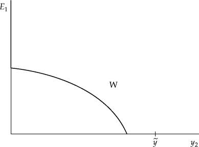
Fig. 5.4 Graphic representation of equation (5.9) yields W curve.

Source: Aghion et al. (2001), figure 3.

reduces first period profits ∏1 through an increase in the foreign currency debt burden of domestic entrepreneurs.

To conclude this section let us briefly compare our model with a standard open macro model. On the one hand, such a model would include the same kind of IPLM relationship between expec­ted output and the current nominal exchange rate, but on the other hand: (i) our downward-sloping W curve would be replaced by an upward-sloping IS curve (with entrepreneurs' output decisions being constrained by aggregate demand instead of being con­strained by current wealth); (ii) our price rigidity assumption would be replaced by some kind of a Phillips curve that would

fundamentals or to expectations such that Ei = Pi. The W curve has in common with the Phillips curve that it is vertical in the absence of unanticipated shocks.

106 The Third Generation Approach to Currency Crises determine the rate of price adjustment as a function of the other variables of the model. The fact that the W curve slopes down is of course key to our analysis. Consequences of relaxing this assumption will be discussed later. The value of making specific assumptions about price rigidity rather than adopting an omni­bus Phillips curve approach is that it makes clear why different degrees of rigidity can have very different implications for the optimal monetary response to currency crises.

5.2.2 Equilibrium

For a given future path of inflation or nominal interest rates, the equilibrium values of Ei and y2, are determined by the two equations, (5.1) at t = 1 and (5.5), in which ⅛ is taken as given.

The reason for multiple equilibria is simple: if a large cur­rency depreciation is expected, consumers will reduce their money demand because expected output is lower. This in turn leads to a currency depreciation, confirming the consumers' expectations. On the other hand, if no large depreciation is expected, it will not occur in equilibrium because in this case domestic consumers will not reduce their demand for the domestic currency.

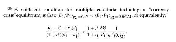
Sufficient conditions for having a multiplicity of equilibria require the W curve intersecting the y2 axis below the IPLM

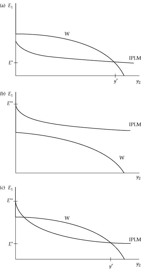
Fig. 5.5 Short-run equilibrium of the model (a) "good"case, (b) "bad"case, (c) "intermediate"case.

Source: Aghion et al. (2001), figure 4.

108 The Third Generation Approach to Currency Crises curve.²⁶ A currency crisis of this type can be set off by a variety of factors. In the case where there are actually multiple equilib­ria, the crisis could be brought on by a pure expectational shift. If everyone believes that there will be crisis, then a crisis occurs.²⁷

On the other hand, in the case where the initial configuration is as in Figure 5.5(a), only shocks to fundamentals can bring on a crisis.

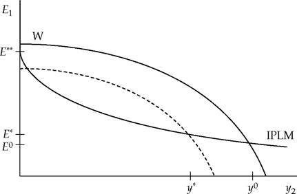
Fig. 5.6 Shock to fundamentals with possible currency crisis. Source: Aghion et al. (2001), figure 5.

²⁷ It is possible to show that these multiple outcomes can also occur when expectational shifts are taken into account when setting prices (formally, in Aghion et al. (2004b) we derive sufficient conditions for the existence of nondegenerate sunspots equilibria).

either to (y'*, E*) or in the worst case to (0, E**). The latter case corresponds to a currency crisis situation.

Similarly, suppose that, due to a substantial increase in the perceived exchange rate risk the country now has to pay a risk premium on bonds denominated in its currency. In this case the interest-parity equation (5.1) becomes:

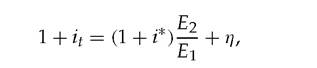
where η is the foreign exchange risk premium after the shock.^[34] This increase in risk shifts the IPLM curve upwards, as the new IPLM equation becomes:

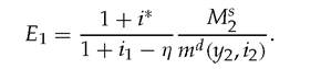
Starting from a “good case"situation with only one equilibrium with low E1 and high y2, this upward shift in IPLM may again lead to a multiple equilibria situation, and therefore to the possibility of a currency crisis. This possibility is actually reinforced by the fact that an increase in the foreign exchange premium raises the interest rate on foreign borrowing which in turn will tend to move the W curve downward.

Similar effects would also follow from an increase in country risk. This leads to an increase in the interest rates faced by domestic entrepreneurs both with regard to domestic and foreign currency debt obligations. An increase in the country risk premium would thus shift the W curve downward without affecting the IPLM curve. In the next section we examine the effects of shocks induced by fiscal and/or monetary policy.

5.3