The basic model

A more fully-fledged and microfounded version of the model in this section is developed in Aghion et al. (2004b). While we chose

96 The Third Generation Approach to Currency Crises to present a reduced form version for pedagogical purposes, we highly encourage the reader to then move to the microfounded version which also contains a more elaborate policy discussion.

We consider an infinite-horizon small open economy monetary model where goods prices are determined at the beginning of each period and remain fixed for the entire period.¹² There is a single tradable good and purchasing power parity (PPP) holds ex ante, that is, P_t = E^e_t for each t, where P_t is the domestic price set by firms, E^ιe is the expected nominal exchange rate (the price of foreign currency in terms of domestic currency) at the beginning of period t, and the foreign price is constant and equal to 1. Prices are preset for one period.

A key ingredient of our model will be a shock in period 1 that occurs after the price in that period has been set. This shock may be real—such as a change in productivity or competitiveness or the risk perceptions of bondholders at home or abroad. Or it may be a pure shift in expectations—as is well-known, in a world of multiple equilibria, such shifts can have real effects.¹³ The shock causes a deviation from PPP ex post in period 1, that is¹⁴:

Since prices cannot move during period 1, the nominal exchange rate has to move to absorb the shock.^[27] These deviations will play a crucial role in the analysis.

¹² The assumption that prices are preset for one period is commonly made in monetary models of an open economy, following Obstfeld and Rogoff (1995).

¹³ For most of the chapter we assume that the shock is wholly unanticipated and is not taken into account by the domestic market when setting the date-1 price. This assumption is commonly made by the existing models of open monetary macroeconomics (see again Obstfeld and Rogoff, 1995). However, our results hold when the distribution of expectational shocks is taken into account ex ante, as shown in Aghion et al. (2004b).

¹⁴In Aghion etal. (2004b) we concentrate on the existence of rational expectation sunspot equilibria in which P₁ is equal to the expected exchange rate in period 1, that is:

The analysis in this chapter relies in a fundamental way upon two basic assumptions about credit markets. First, we assume that credit markets are imperfect. As in the previous chapters, entre­preneurs cannot borrow more than a fixed multiple mw_t of their current real wealth w_t. Entrepreneurs' wealth thus remains the fun­damental state variable that determines investment and output. Second, we assume that firms hold foreign currency debt, whose servicing cost for domestic borrowers thus varies with the nominal exchange rate. This in turn introduces the pecuniary externality part of the story.

While this latter assumption accords well with what we observe in many emerging market economies, it requires a justification. In Schneider and Tornell (2000) foreign currency borrowing fol­lows from the assumption that domestic banks are bailed out by the government in case of default, so that firms will want to increase their risk of exposure by borrowing in foreign currency. Jeanne (2000a,b) develops models in which foreign currency bor­rowing serves as a signaling or as a commitment device. In Chamon and Hausmann (2002) and Aghion et al. (2001) foreign currency borrowing follows directly from extrinsic exchange rate uncertainty together with the assumption that the currency com­position of a borrower's portfolio is not contractible: in that case, if a first lender decided to lend in domestic currency, the borrower could use the amount of the loan as a collateral to borrow from a second borrower in foreign currency; then, a large currency depre­ciation together with limited liability would allow the borrower to (partly) default on the first lender.

In all other respects the model is quite standard: output is pro­duced using capital, and the production function y_t = f (k_t) has the standard concave shape. There is full capital mobility, and uncovered interest parity holds. The exchange rate can be either floating or fixed, even though the fixed exchange rate case is only explicitly analyzed in Section 5.3. Consumers need money for their transactions, and there is a central bank that can alter interest rates or the exchange rate by affecting money supply.

The timing of events can be summarized as follows. In the first period, the price P₁ is preset and firms invest. Then, an unanti­cipated shock occurs followed by a monetary adjustment which determines both the nominal interest rate iι to be paid at the end of the second period (interest rates are always set one period ahead) and the nominal exchange rate Ei (when the latter is not maintained fixed). Subsequently, period 1's output and profits are generated and firms' debts are repaid. Finally, a fraction (1 — α) of net retained earnings after debt repayment, namely w2, is saved for investment in period 2.^[28] Periods after period 1 are identical in all respects except in that after period 2, no further shock occurs and the economy converges to its steady state.

The remaining part of this section, first, describes the monet­ary side of the economy and, second, analyzes the entrepreneurs' borrowing and production decisions.

5.1.1 The monetary sector

The interaction between consumers, foreign investors, and the central bank gives us both a money market equilibrium con­dition (i.e. an LM curve) and an interest parity (IP) condition (i.e. an IP curve). Since both types of conditions are standard in open economy macroeconomics, we shall not expand on their microfoundations.^[29] Arbitrage by investors between domestic and foreign currency bonds in a world with perfect capital mobility yields the following IP condition:

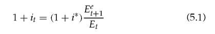
where i* is the foreign interest rate which we assume to be constant over time.

In addition, consumers have a standard real money demand function m^d = m^d (y_t, i_t). The function m^d has the usual proper­ties of being increasing in y_t and decreasing in i_t;^[30] furthermore,

When crises are anticipated, the key issue is whether the endo­geneity of currency exposure would eliminate the possibility of a crisis. Note that when the borrower chooses the currency compos­ition of his own debt, he takes as given the composition of debt in the rest of the economy—he will not deviate from his privately optimal choice of currency composition to prevent a crisis. He may have private reasons for preferring domestic currency debt if there is some chance of a crisis, especially if default is costly for him. However, given that he cannot prevent the crisis by making this choice, moving to domestic debt simply shifts the risk on to the lender, who will accept it only if the price the borrower pays for the insurance (in terms of foregone benefits from holding foreign currency debt as well as the cost of compensating the lender for the extra risk he bears) is worthwhile; this would only be the case if a crisis were sufficiently likely. It follows that if all the other borrow­ers were to choose levels of d_t^c that are such that no crisis is possible, an individual borrower would simply choose the level of domestic currency debt, d^c_t, that is optimal for him without the possibility of a crisis. If this preferred level of foreign currency debt happens to be higher than the minimum needed to make a crisis possible, the only equilibrium value of d_t^c is one where there will sometime be a crisis. Note that this reasoning is valid independently of the reason for which borrowers hold foreign currency debt.

Given the currency composition of domestic entrepreneurs' debt, we can now express their aggregate nominal profits net of debt repayments at the end of any period t, namely:

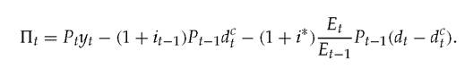
Whenever profits are positive, entrepreneurs retain a proportion (1 — α) of profits and use them to finance their future investment (a proportion α of profits is distributed and/or consumed).

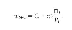
It follows that second period output y2, which is a function of the wealth W2 available at the beginning of period 2, is given by:

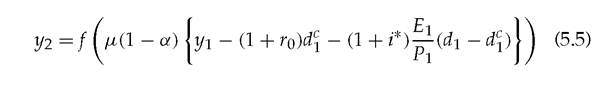
where ro is the real interest rate defined as 1 + r_t = (1 + i_t)P_t∕P_t+1 and 0 < y2 < y. Equation (5.5) clearly shows that output would react negatively to an increase in the debt burden induced by a cur­rency depreciation, that is by an increase in E1. Note that changes in the nominal interest rate i₁ do not affect the debt burden in period 1 and output in period 2. The reason is simply that i1 is the interest rate applying to the second period.

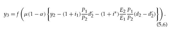
However, i₁ will affect the cost of domestic currency debt and therefore the debt burden in period 2 positively, and therefore the output in period 3 negatively. More formally, we have:

In any period t ≥ 3, the PPP condition continues to hold but in addition the discrepancy between E₁ and P₁ no longer affects the total debt burden of entrepreneurs, that is, domestic and foreign currency debt become fully equivalent. Hence, for t ≥ 3 output yt+1 is simply given by:

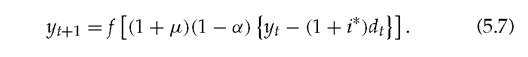
The model is now fully laid out. Equilibrium in this model is defined as a sequence of prices (P_t), exchange rates (Et), and output levels (y_t), which for a given monetary policy in period 1 satisfy the above equations (5.1)-(5.3), (5.5), and (5.7) for all t. The dynamics of aggregate output y_t for t > 2, are easy to com­pute and can be simulated numerically. However, a diagrammatic presentation offers more insight into the nature of the equilibrium and is presented in the following section.

5.2