Self-organizing Patterns of Consumption
So far, we have confined the objects of analysis to a closed domain, to permit a mathematically complete analysis. Once the domain equipped with the desired properties is built up, the analysis will succeed, providing we have sufficient mathematical skill.
Here “domain” may be interpreted as “environment”. In this sense, traditional economic thinking may be classified as “environmentalism”. However, in reality, human satisfaction and consumption cannot be confined to a particular closed space. The space is always exposed to the external environment and its fluctuations. The resulting consumption pattern may be considered as a selforganizing activity affected by the outer world. The idea of mathematical closedness both in the commodity space and in terms of personal satisfaction must be a fallacy, if we envisage the way in which patterns of consumption form in reality. Outside sophisticated mathematical modeling, we need a different idea of consumption.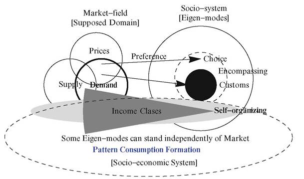
Fig. 2.8 Evolving satisfaction and the formation of a pattern of consumption
2.3.1.1 Formation of Patterns of Consumption
The formation of patterns of consumption is shown in Fig. 2.8. Market field is the domain supposed by traditional economics, a hypothetical reference. The link between price and demand is intermediated by the substitution and income effects. The income effect is no longer fixed outside different income classes, known as “the socioeconomic system”. An actual pattern of consumption will appear in the range of two domains, i.e., the socioeconomic system. This section sets out the formation of the pattern of consumption.
We can easily obtain the yearly income of all households of five income rank classifications, with monthly receipts and disbursements per household, for instance.11 Table 2.2 lists ten categories of expenses, and there are five income ranks.
If there are any similar major principal modes, each income class can be derived from empirical data by a spectra distribution, and also be separated explicitly from the derived random distribution by the random matrix theory. It can therefore be verified that there is a common factor over the different income classes, and the effects of macroeconomic variables on the spending categories over the different income classes can be identified.In reality, the members belonging to an income class are constantly changing. A member may fall into a lower income class, or rise to the next one. We assume that the movements between classes cancel each other out because of a limitation [34]
Table 2.2 The categories of expense items
Expense items
1. Food
2. Housing
3. Fuel, light, and water charges
4. Furniture and household utensils
5. Clothing and footwear
6. Medical care
7. Transportation and communication
8. Education
9. Culture and recreation
10. Other
Table 2.3 Mode 1 (eigenvalue A1 = 4.24)
| I | II | III | IV | V | |
| 1 Food | 0.288 | 0.275 | 0.281 | 0.283 | 0.335 |
| 2 Housing | -0.069 | -0.070 | -0.024 | 0.034 | 0.018 |
| 3 Fuel, light and water charges | 0.088 | 0.193 | 0.189 | 0.161 | 0.128 |
| 4 Furniture and household utensils | 0.137 | 0.091 | 0.067 | 0.153 | 0.030 |
| 5 Clothing and footwear | 0.086 | 0.264 | 0.058 | 0.161 | 0.176 |
| 6 Medical care | 0.049 | -0.059 | 0.115 | 0.109 | -0.032 |
| 7 Transportation and communication | 0.098 | 0.083 | -0.056 | 0.169 | 0.005 |
| 8 Education | 0.005 | -0.088 | 0.035 | -0.160 | 0.071 |
| 9 Culture and recreation | 0.141 | 0.171 | 0.071 | 0.043 | 0.171 |
| 10 Other | -0.056 | 0.096 | 0.094 | -0.019 | 0.122 |
Note: The data used are from Jan 2000 to Feb 2012
of statistical data. Types are then replaced with state variables.
Hildenbrand (1994) called this assumption metonymy.The sample numeric space is therefore given by five income classes x 10 household expense items x the number of months. By deriving the correlation matrix, we can calculate its eigenmodes and which components are constituted by the items of consumption. Each income class has its own eigenmode, as Table 2.3 shows. We may then call the eigenmode “the pattern of consumption”. By comparing the eigenvector component sizes corresponding to the expense items in this mode, and common to different classes, we see that FOOD is the dominant factor. This mode could then be called the FOOD-dominant mode. The FOOD item is paired with the remaining items. Spending on these factors may move with FOOD spending as the consumption level varies. This mode indicates a pattern of consumption around FOOD.
In the next subsection, we will see an independent force separated from a supposed market field. A new tool can be used to identify a nonrandom eigenmode among those of a socioeconomic system, and across the whole period under investigation. We will apply random matrix theory to sample data to empirically verify that some eigenmodes could be judged as nonrandom independently of a hypothetical market field.
2.3.1.2 A Force Common to All Income Classes
Before checking the empirical properties of patterns of consumption in Japan, it may be helpful to sum up two distinct forces:
1. A force to cancel out irregularities in demand direction: class differences may contribute to mitigate irregularities, as Hildenbrand (1994) noted (see Sect. 2.2).
2. A force to create a self-organizing assimilation of a segmented consumption basket, whether partly class-specific or common to all classes. Some independent forces may work the same way across all classes rather than differently for different classes.
2.3.2