Some illustrative theory
4.1. The Green Solow benchmark[499]
Every model relating economic growth to emissions or environmental quality has by construction made implicit assumptions regarding the strength of scale, composition and technique effects.
These assumptions are often hidden in choices made over functional form, over the number of goods, the inclusion of finite resources, or in assumptions concerning abatement. Since we have data on the composition of output, its scale, and emissions per unit of output, it is often useful to divide models into categories according to their reliance on scale, technique and composition effects rather than model specifics like the number of goods, types of factors or assumptions over abatement. By dividing up the literature along these lines, we can weigh the relative merits of model’s that rely exclusively on composition effects by looking at their strength in the data rather than by asking ourselves far less obvious questions such as are capital and resources good or poor substitutes or does abatement exhibit increasing returns.The literature linking growth and pollution levels is immense starting with very early work in the 1970s by Forster (1973), Solow (1973), Stiglitz (1974), Brock (1977) and others, and culminating in the more recent work investigating the Environmental Kuznets Curve such as Stokey (1998), Aghion and Howitt (1998), or Jones and Manuelli (2001). Although the earlier and late literatures differ greatly in their assumptions regarding the driving force behind growth, all models of economic growth must produce changes in scale, composition, or techniques that satisfy (1). Models that produce similar aggregate relationships between income and pollution often rely on different mechanisms to drive pollution downward. Because of these differences, they have other observable implications that we can use for evaluation.
To start our enquiry into the various mechanisms authors have employed to generate sustainable growth or an EKC prediction, we develop an augmented Solow model where exogenous technological progress in both goods production and abatement leads to continual growth with rising environmental quality. This is the simplest model to explore the importance of technological progress in driving down emissions per unit of output.
Consider the standard one sector Solow model with a fixed savings rate s. Output is produced via a CRS and strictly concave production function taking effective labor and capital to produce output, Y. Capital accumulates via savings and depreciates at rate S. We assume the rate of labor augmenting technological progress is given by g. All this implies
To model the impact of pollution we follow Copeland and Taylor (1994) by assuming every unit of economic activity, F, generates Ω units of pollution as a joint product of output. The amount of pollution released into the atmosphere may differ from the amount produced if there is abatement. We assume abatement is a CRS activity and write the amount of pollution abated as an increasing function of the total scale of economic activity, F, and the economy’s efforts at abatement, Fa. If abatement at level A, removes the ΩA units of pollution from the total created, we have
where the third line follows from the linear homogeneity of A, and the fourth by the definition of θ as the fraction of economic activity dedicated to abatement.
The relationship in (14) requires several comments. The first is simply that (14) is a single output analog of (1) showing that emissions are determined by the scale of economic activity F, and the techniques of production as captured by e(θ).
The second is that the production of output per se and not input use is the determinant of pollution. Since there is only one output, this means the composition effect must be zero. In a subsequent section we alter our formulation to consider pollution created by input use, but note in passing here that making pollution proportional to the employment of capital has no effect on our results. Finally, since Fa is included in F, even the activity of abatement pollutes.To combine the assumptions on pollution in (14) with our Solow model, it is useful to assume the economy employs a fixed fraction of its inputs - both capital and effective labor - in abatement. This means the fraction of total output allocated to abatement θ is a fixed much like the familiar fixed saving rate assumption.33 As a result, output available for consumption or investment Y, becomes [1 - θ ]F. In addition we must adopt some assumption concerning natural regeneration. To do so we assume the quality of the environment evolves over time according to (6). Therefore, the evolution of environmental quality is given by

Finally, since the Solow model assumes exogenous technological progress, we assume emissions per unit of output fall at the exogenous rate gA. Putting these assumptions together and transforming our measures of output and capital into intensive units, our amended Solow model becomes:
[1] We treat θ as endogenous when examining transition paths in Section 5. It is possible that no abatement is optimal in some limited circumstances, but in models generating balanced growth this would imply every increasing pollution levels. In models without growth, such as Keeler, Spence and Zeckhauser(1972), a Murky Age or Polluted Age equilibrium result is possible with θ set to zero.
Technological progress in abatement must exceed that in goods production because of population growth; and some technological progress in goods production is necessary to generate per capita income growth.
The Green Solow model, although very simple, demonstrates several important points. The first is that investments to improve the environment may cause only level and not growth effects. This is obviously true here since the growth rate of per capita magnitudes is explicitly linked to the rate of technological progress, but not to θ. By setting the time derivative of capital per effective worker to zero in (16) it is straightforward to show that a tighter environmental policy (higher θ) lowers output, capital and consumption per worker, but has no effect on their long run growth rates.
The implied income and consumption loss from a tighter policy is however quite small. Adopting a Cobb-Douglas formulation for final output with the share of capital equal to α shows that the ratio of consumption per person along the balanced growth paths of the economy adopting weak versus strong abatement is just

since both economies grow at rate g + n. If weak abatement means adopting a share of pollution abatement costs in national output of 0.5%, and strong abatement means 10%, then consumption per person will differ by 16% along the balanced growth path (assuming capital’s share in output is 0.35). Therefore, a twenty-fold difference in the intensity of abatement creates only a 16% difference in consumption per person!
The calculation however seems to imply that environmental policy cannot be much of a limit on economic growth. Recall though that for any given choice of abatement intensity, if we are to have ongoing growth, an improving environment, and a constant (relative) cost of environmental policy, then technological progress in abatement must be sufficiently strong.
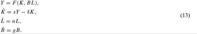
This is clear from (17) which we can interpret and saying that sustainable growth in income per capita is only possible at the rate of technological progress in abatement. If technological progress is slower than that given in (18) then one of two things must happen. Either additional investments in abatement are undertaken to maintain environmental quality, or environmental quality must decline. At this point however we should note that the strict concavity of A implies there are diminishing returns to greater and greater abatement efforts. From (14) we find that e'(θ) = -A2 < 0, but e"(θ) = -A22 > 0. Therefore, in the absence of strong technological progress in abatement, growth in income per capita is only consistent with lower pollution levels if abatement grows over time.[500]One final observation concerns the transition path of the model. Despite the fact that environmental policy is fixed and there are no composition effects in our one good framework, simulations of the Green Solow model produce a path for income and environmental quality tracing out an Environmental Kuznets Curve. This surprising result
Figure 9. The Green Solow benchmark.
is shown graphically in Figure 9, where we present the trajectories for two economies that are identical in all respects except for their abatement intensity. Each starts from an initially pristine environment and a small initial capital level. Strong abatement refers to a 10% share of output spent on abatement; weak abatement to a 0.5% share. The other parameters were chosen for the purposes of illustration. Per capita income grows at 1% along the balanced growth path, the population grows at 2% and the abatement technology improves at 5%. Note that these parameters ensure that growth is sustainable according to (18). Capital’s share is set at 0.35, the savings rate is 10% and depreciation is 2%.
Regeneration is set with η = 0.1 implying a 10% rate for any X > 0.As shown, the environment at first worsens and then improves as the economy converges on its balanced growth path. Note that along the balanced growth path emissions fall and the environment improves at 2% per unit time, which is close to what the simulation delivers in its last periods.
This result follows for three reasons. First, the convergence properties of the Solow model imply that output growth is at first rapid but then slows as k approaches k*. With a fixed intensity of abatement, pollution emissions grow quickly at first but slower later. Therefore, part of the dynamics is governed by the convergence properties of the neoclassical model.
Second, when we start at a pristine environment the effective rate of natural regeneration is zero. This is true because “nature” is at a biological equilibrium with X = 0. When production begins the environment deteriorates. At X = 0, the introduction of any emissions overwhelms the rate of regeneration and lowers environmental quality. As X rises, natural regeneration rises. This must be a feature of the regeneration function in order for X = 0 to be a stable biological equilibrium.
Third, we have assumed emissions fall along the balanced growth path.
Together the first two facts imply that at the outset of economic growth the rapid pace of growth swamps nature’s slow or zero regeneration; but the economic growth rate slows and regeneration rebounds. As we approach the balanced growth path natural regeneration must overwhelm the now less rapid inflows of pollution. The environment improves.
It is important to recognize that this result is more general than our Cobb-Douglas technology and instead relies on quite general properties of production and growth functions. To verify write the dynamic system governing k and X as

35 With a further assumption on technology we can ensure the EKC must be single humped. Our Cobb- Douglas formulation adopted in the figure is covered by our assumption. per person and consumption per person both fall with increases in θ while pollution is lowered. Forster’s work is important because it was perhaps the first examination of optimal pollution control in a neoclassical setting.
The Green Solow model is also similar to the neoclassical model adopted in Stokey (1998), but differs in that Stokey gives no role to technological progress in abatement. As a result increasing abatement intensity must carry the day in reducing pollution. Stokey also generates the EKC prediction but her result follows from a change in pollution policy along the transition path. Her simulations of the model must reflect the dynamic forces we have identified since the model is neoclassical and the evolution equation for the environment is identical.
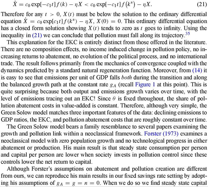
More closely related work is Bovenberg and Smulders (1995). In their endogenous growth formulation “pollution augmenting technological progress” holds pollution in check and drives long run growth. In their two-sector model, ongoing investments in the knowledge sector raise the productivity of pollution leading to a balanced growth path with a constant level of environmental quality. Again our Green Solow model reproduces the flavor of their results. Setting n = 0 to mimic their zero population growth assumption, and assuming g = gA to mimic the identical rates of technological progress found in both sectors, we find from (22) that emissions are constant along the balanced growth path and output per person grows at rate g.
This similarity should not be all that surprising because Bovenberg and Smulders’ “pollution augmenting technological progress” is very similar to our technological progress in abatement. To see why divide both sides of our emissions function in (14) by Ω, and then employ the monotonicity of A in θ to invert the intensive abatement function and solve for [1 - θ]. Use this to write net output Y = F[1 - θ] available for consumption or investment as
4.2. Intensifying abatement: the Stokey alternative
We now amend our Green Solow model to incorporate a role for an active environmental policy. In the model above reductions in pollution came about solely because of changes in the emission technology and not because society allocated more resources to pollution prevention. InanimportantpaperNancy Stokey [Stokey (1998)] presented a series of simple growth and pollution models to investigate the links between the limits to growth and industrial pollution. She examined the ability of these models to reproduce the results of empirical work finding an Environmental Kuznets Curve and investigated how an active environmental policy may place limits on growth. An important feature of Stokey’s analysis was its dependence on increased abatement and tightening regulations to drive pollution downward.
Her analysis contains two contributions. The first is a simple explanation for the empirical finding of an Environmental Kuznets Curve. Like Lopez (1994) before her, and Copeland and Taylor (2003) after, Stokey shows how an income elastic demand for environmental protection can usher in tighter regulations and eventually falling pollution levels. This assumption on tastes, together with certain assumptions on abatement, succeeds in generating a first worsening and then improving environment as growth proceeds.
Stokey’s second contribution was to investigate whether there are limits to growth imposed by regulating industrial pollution. In Section 5 we discuss her analysis within an AK framework; here we focus on her work within the neoclassical model that formed the bulk of her paper. To do so we make the smallest departures possible from the Green Solow model. We again take the savings rate as fixed, but allow the intensity of abatement to vary over time. Since we are primarily interested in feasibility rather than optimality, our fixed savings rate assumption will simplify the analysis with little or no cost. Stokey assumed zero population growth, exogenous technological progress in goods production, a Cobb-Douglas aggregator over capital and labor in final goods production, and adopted an abatement function drawn from Copeland and Taylor (1994). In Stokey’s analysis an optimizing representative agent determine savings and abatement decisions.
Although it is not obvious from Stokey (1998), a process of pollution abatement is implicit in her analysis. In Stokey’s formulation the planner chooses a consumption path and the techniques of production as indexed by “z”. The choice of techniques determines the link between potential output, F, and final output Y available for consumption or investment. The two are related by Y = Fz; while aggregate emissions are given by E = Fzβ for some β > 1. To see how this choice of “techniques” is really one over abatement intensity make the change of variables (1 - θ ) = z, and then let e(θ) = (1 - θ )β for β > 1. It is now easy to see that the “techniques” chosen by the planner correspond to choices over the abatement intensity θ. The resulting e(θ ) is just a specific form of an emissions function coming from the assumptions of constant returns to abatement and pollution being a joint product of output. Since θ is in principle observable, we conduct our analysis in this unit.
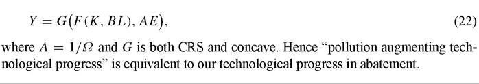
Our amended model assumes zero technological progress in abatement, and to follow Stokey adopts the specific emissions function given above and a Cobb-Douglas aggregator over factors. The model is described by:
To examine the feasibility of balanced growth with a nondeteriorating environment we start with the last equation in (23) giving emissions and log differentiate to find
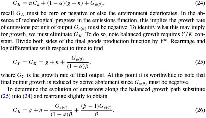
The first two terms of this expression, (n + g), represent the scale effect of growth. They represent the growth rate of emissions that would arise along the balanced growth path if θ and hence environmental policy, was held constant. This is clear from (23) since if θ is constant Ge(θ) — 0.
The final two terms in (26) represent the technique effect created by lowering emissions per unit output along the balanced growth path. This technique effect is itself composed of two parts. The first component is the reduction in the growth rate of final output caused by the diversion of resources to abatement. Since θ is increasing along the balanced growth path, the growth rate of F exceeds that of final output by this amount.[501] Therefore, this component of the technique effect lowers pollution by slowing down the growth rate of final output [recall (25)].
The second component of the technique effect is the reduction in emissions per unit of final output created by abating more intensively. This is the standard component identified in static models. This component of the technique effect need not be as large as previously to lower pollution. To see this solve (26) for the rate at which emissions per unit of output must fall to drive emissions downward. Algebra yields

which is smaller than the minimum rate of (g + n) needed in (17). Not surprisingly because abatement has a negative effect on growth rates, it has less of a role to play in lowering emissions per unit of output. Therefore in set-ups where abatement is responsible for pollution reduction, the burden is shared across two margins: abatement lowers growth rates and abatement also lowers emissions per unit output.
These two roles for abatement now introduce the possibility that a sustainable growth path may not exist. To see why, note that the reduction in growth created by environmental policy is very similar to the growth drag found in models with either fixed land or exhaustible natural resources.[502] In the case with fixed or declining resources the ratio of resource use to effective labor falls along the balanced growth path and this lowers growth rates. The same is true here once we make the right translations. To see this parallel, use the final goods production function and the emissions function to write net output as if pollution were an input into production. Doing so we find

Along the balanced growth path E must fall while F grows; therefore the reduction in E works very much like the exhaustion of a resource that lowers growth. It is now apparent that while (27) tells us that the decline in emission intensity must be sufficiently fast to lower emissions; Equation (25) tells us this same magnitude cannot be too large if we are to have positive growth in income per capita. Solving (25) for the implied restriction and combining with (27) yields, after some manipulation,

The range given by this inequality defines the set of emission intensity reductions that are consistent with declining emissions and positive per capita output growth: i.e. sustainable growth. If we recall that β > 1, then it is straightforward to see that the feasible region is not empty when there is zero population growth. When n > 0 the region may not exist. By equating the two sides of (29) we can solve for the relationship between population growth and parameters that must be true for a sustainable growth path to exist. Algebra gives us

The left-hand side of (30) is exactly labor’s share in final goods production [use (28) and the definition of F] times the rate of labor augmenting technological progress g. The right-hand side is exactly emissions share in final output, 1∕β, times the rate of population growth n. The intuition for this condition is straightforward, and is identical to that we give later in a model where exhaustible energy resources create drag.
The left-hand side of the expression represents the Solow forces of technological progress raising growth to the extent determined by labor’s share and the rate of progress. The right-hand side could be called the Malthusian forces since they capture the impact of diminishing returns caused by a falling ratio of emissions to effective labor along the balanced growth path. These forces are stronger the more important are emissions in the production of final output, and stronger the faster is population growth.
If the inequality in (30) goes the other way then we have two choices. Either per capita income growth is negative and emissions fall; or, per capita income growth is positive but emissions rise. In either case we do not have sustainable growth according to our definition.
This observation of course suggests we follow the path of earlier authors and calculate the growth drag due to pollution policy. For example, Nordhaus (1992) adopts a model similar to (28) with emissions E replaced by either land or an exhaustible natural resource and then generates estimates for the drag caused by finite land and natural resources. But without a formal framework in which to estimate the long run growth impact of tighter environmental policy, Nordhaus resorts to estimates of contemporaneous expenditures on abatement to calculate future costs of pollution control.
We can go further here, although our methods are far from ideal. To generate an estimate for the growth drag caused by environmental policy we need estimates of β, α and Ge(θ). We note using (23) that Ge(θ) = GE/Ye/[e — 1] where GE/Y is the observable growth rate of emissions per unit of final output. For various measures of E it is shown in Figure 1. We take capital’s share of production, α to be 0.35. To eliminate the parameter β write emissions per unit of output, using (23) as E/Y = (1 — θ)β—1. Since we have data on emissions, final output and pollution abatement costs we could in theory estimate β. Using this estimate we could then calculate the growth drag due to pollution policy. Since our purpose is not to provide definitive answers but rather suggest a methodology, take the log of E/Y and differentiate with respect to time to find

where Ge is the growth rate of the pollution abatement cost share, and θ the average pollution abatement cost share over the period in consideration. Now use (31) to eliminate β and now rewrite (25) as

The drag due to environmental policy is now directly linked to observable measures: the share of pollution abatement costs in the value of overall economic activity, and the percentage growth rate of this measure. To investigate what a reasonable magnitude of growth drag may be, we report in the table below a series of illustrative calculations. Recall that the share of pollution abatement costs in either manufacturing value-added or GDP is small - on the order of 1 or 2%. In certain industries it can of course be much higher. Take 1970 as the base year and set the pollution abatement costs share in that year at 1%. Then applying growth rates of 2.5 to 7.5% per year in this cost share, we obtain with the help of (32), the following results.
The first column of Table 1 assumes the share of pollution abatement costs in the value of output rises from 1% to a little over 2% in thirty years. The other columns report larger increases for illustrative purposes, although they are far in excess of the historic increases as shown by our data in Figure 2. A striking feature of the table is that the drag due to environmental policy is very small except in extreme cases. When pollution abatement costs rise from 1% to a little over 2% in 30 years, the drag on growth is only 6 hundredths of 1% point. When pollution abatement costs grow by 5% per year, the policy reduces growth by 0.2%. If costs grow by the extremely large 7.5% per year, drag is now 2 of 1% point which is significant. Note that growth in per capita income, Gy — n, over the last 50 years is approximately 2% per year; therefore the last column would predict an ever strengthening environmental policy that raise the share of pollution abatement costs in value-added by 7.5% year would reduce per capita income growth by 25%.
To a certain extent the relatively small effects in Table 1 are not that surprising. If pollution abatement costs as a fraction of value-added are in the order of 1%, it is difficult to see how even relatively large percentage increases in their level would lower growth tremendously. To go slightly further, note from (31) that if Ge∕y and Gθ are of the same magnitude, then it is easy to see that β is approximately 1∕θ.[503] This implies the share of emissions in final production in (28), 1 /β is on the order of 0.01 or 0.02. And if pollution emissions are such an unimportant input into the production of final output, then drag from any reduction in emissions over time must also be small.
Despite the optimistic results in Table 1 concerning growth rates, models that rely on active abatement often contain the prediction that abatement becomes a larger and larger component of economic activity. This is a direct consequence of two facts. The first is that for emissions to fall, emissions per unit of output must shrink continuously with ongoing growth. The second is that with constant returns to abatement, lowering emissions per unit output comes at increasing cost. As a consequence, an implication of an exclusive reliance on abatement is that abatement costs rise along the growth path to eventually take up most of national product. To verify this, return to our simple example
Table 1
The drag of pollution policy on growth (percentages)
| PAC share percentage increase per year | 2.5 | 5.0 | 7.5 |
| Pollution abatement costs share 1970 | 1.0 | 1.0 | 1.0 |
| Pollution abatement cost share 2000 | 2.1 | 4.3 | 8.8 |
| Average θ∕[1 — θ] across period | 1.57 | 2.72 | 5.15 |
| Growth drag percentage | 0.06 | 0.2 | 0.5 |
and note Ge(θ) is constant along the balanced growth path. Using our specific emission function in (23), we know

Solving this differential equation for θ yields

starting from some θ(0) near the balanced growth path we see that as time goes to infinity θ goes to one because Ge(θ) < 0. Abatement must take up a larger and larger share of national product as time progresses. This is an uncomfortable conclusion in light of the data we have already presented showing a relatively weak increase in abatement over time. In addition the reader may wonder why it is that agents would willingly make such sacrifices in final consumption necessary for such a large abatement program.
At this point it is useful to refer to Stokey (1998) explicitly for an answer since Stokey’s analysis shows that consumer’s are indeed willing to make the sacrifice needed in net output to lower pollution albeit under certain conditions. Specifically, by adopting a CRRA utility function Stokey shows emissions fall along the balanced growth path if and only if the elasticity of marginal utility with respect to consumption exceeds one. Only if consumers valuation of consumption falls quickly are they willing to take a smaller and smaller slice of (an ever expanding) national income as growth proceeds.
Stokey’s analysis also allows for a more theoretically based growth drag calculation. By adopting specific functional forms, Stokey solves for the growth rate of final output and emissions in terms of primitives. By rearranging slightly and recasting these results in terms of our notation we find the growth rate of output per person and overall emissions are just
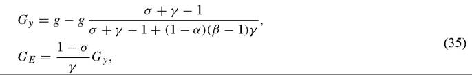
where σ is the elasticity of marginal utility in the CRRA utility function, γ f 1 is a measure of the convexity of damages from pollution, α is capital’s share, g is the exogenous rate of labor augmenting technological progress. There is zero population growth so n = 0.[504]
In comparison to our simple example the drag of environmental policy is now directly linked to the primitives of tastes and technology although it reflects similar forces at work. For example, by rearranging we can isolate the percentage reduction in growth
caused by active pollution policy

the greater is the rate of reduction in emissions per unit output, Ge∕y, and the larger is emissions share in final output 1∕β,the greater will be the drag. This is the same set of forces we found using our simpler framework.
We can of course estimate growth drag in this optimizing framework as well. In order to replicate the Environmental Kuznets Curve Stokey adopts a set of parameters for all the primitives we need. In doing so, the model predicts the EKC found in empirical work, but using these same values for capital’s share, the abatement technology, etc. we find that growth drag is an unbelievable 60% of potential growth. Using the parameter specification chosen to mimic the EKC, growth in income per capita in the absence of pollution policy is 4%peryear.[505] Butusing (35) growth is actually approximately 1.6% per year with active pollution policy; therefore, growth in income per person is slowed by 60% from what it would be in the absence of environmental concerns. This is clearly far too high.
If we lower the elasticity of marginal utility to approach the lowest limit consistent with falling pollution (σ approaching 1), and set γ = 1, then drag hits its minimum. But even in this case, drag is almost 55% of potential growth. The problem with these calculations is Stokey’s assumption of β = 3, which implies a share of pollution emissions in final output of 1 /3 which is clearly far too high. Altering β to values similar to those used in our growth drag calculations suggests a much smaller drag.
For example, from Figure 1 it is apparent that 3 of the U.S. criteria pollutants had an emissions per unit of output in 1998 that were just 1 /10 of their value in 1940. This implies a growth rate of approximately -4% per year from these pollutants. Assuming the share of emissions in final output is 0.02, β is 50, and with a capital share of 0.35 we find the percentage reduction predicted by (36) to be just 0.03. Therefore a 2% growth rate would be reduced to just 1.94% because of the drag of environmental policy.[506]
We would hasten to add however that these calculations are purely for illustration. They demonstrate how the growth drag due to environmental policy may be calculated from primitives on technologies, abatement costs, knowledge of historic growth, and emission levels. We leave it to future research to develop and refine these methods to generate estimates of the growth drag due to environmental policy.[507]
Many other papers rely on an active role for abatement in lowering pollution levels, and therefore must contain predictions for both the drag of environmental policy and the evolution of pollution abatement costs over time. In some work, abatement is specified differently so that it escapes diminishing returns by assumption. For example, early work by Keeler, Spence and Zeckhauser (1972) examines no growth steady states and assumes foregone output is the only input into abatement. As a result of this assumption, marginal abatement costs are constant in their formulation. Even with constant marginal abatement costs they find that when abatement is not very productive a “Murky Age” equilibrium arises: abatement is not undertaken and emissions are high in the steady state. Alternatively, when abatement is very productive in reducing emissions, the steady state is given by a Golden Age equilibrium with active abatement and lower emissions.
Other related work appears in Lopez (1994) and Copeland and Taylor (2003). In these contributions an optimizing social planner chooses the optimal level of abatement but factor supplies and technology are taken as parametric in their exclusively static analyses. Both adopt formulations where abatement is a constant returns activity using conventional inputs and examine how once for all growth in either technology or factor endowments affect pollution levels.43 When growth is fueled by neutral technological progress, Copeland and Taylor show that emissions fall with this source of growth if the elasticity of marginal damage from pollution exceeds one. In a CRRA framework this corresponds to the condition Stokey derived of σ > 1.
In contrast when growth occurs by primary factor accumulation alone, then Lopez (1994) shows that whether pollution rises or falls now depends on both the elasticity of substitution between factor inputs and the income elasticity of marginal damage. If the elasticity of substitution between primary factors and emissions is large, then emissions fall quite easily. When production is Cobb-Douglas, Lopez’s condition is identical to that of Stokey and σ > 1 generates the result that emissions fall with growth.
Together these contributions demonstrate that an improving environment and rising incomes are surely feasible in a standard neoclassical model where abatement is a constant returns activity. This path is also optimal under certain conditions. But by relying exclusively on changes in the intensity of abatement to lower pollution levels consumers must be willing to make rather large sacrifices for a cleaner environment over time. It is in fact this rather large willingness to sacrifice for a cleaner environment that leads to regulation in the first place.
In Stokey (1998), regulation is at first not present as the shadow value of capital is too high and the shadow value of pollution too low when growth begins for the planner to gregative data exercises like the one we just conducted. The results from these studies are quite different. For example, Jorgenson and Wilcoxen (1990) build a 35 industry model of the U.S. economy to estimate the impact of pollution abatement costs and motor vehicle emission standards on overall output and growth. They find that output growth in the U.S. was reduced by almost 0.2% over the 1973-1985 period by these environmental policies, and in level terms U.S. real GDP is lower by a quite significant 2.6%.
43 Lopez (1994) does not present an abatement function per se but it is implicit in his use of the revenue function listing primary factors and emissions as productive factors. allocate any output to abatement. An important input into this decision is that the marginal product of the first unit of abatement is bounded above even at zero abatement.[508] As a result, no abatement is undertaken θ = 0 and pollution rises lock-step with output. Once the environment has deteriorated sufficiently and the now larger capital stock has depressed its shadow value, active abatement begins. There is then a transition period and the economy approaches the balanced growth path described previously.
This explanation for the EKC is very persuasive. It links rising income levels with a lower shadow cost of abatement and a higher opportunity cost of doing nothing. It captures the idea that policy responds positively to real income growth and generates an EKC is a straightforward way. We have already seen however that a further implication of the model is an ever-rising pollution abatement cost share that may be inconsistent with the data. In addition we should note that this explanation predicts a constant emissions to output ratio prior to the regulation phase when emissions are rising. After regulation begins, the emissions to output ratio falls and does so at a constant rate along the balanced growth path [see (35)]. Figure 1 however shows the emission to output ratio was falling long before emissions peaked in Figures 3-8. Therefore, using this data as our guide the model misses entirely the long reduction in emissions per unit output that occurred in the U.S. prior to peak pollution levels being achieved.
These observations suggest, at the very least, that other forces are simultaneously at work and partially responsible for the falling emissions to output ratio and roughly constant control costs in the U.S. historical record. One natural candidate is of course changes in the composition of output towards less energy intensive, and hence less pollution intensive, goods. Much has been made recently about the dematerialization of production and its environmental consequences, and hence we now turn to examine a model relying on just these effects.
4.3. Composition shifts: the source and sink model
There are several ways to escape a worsening environment as economic growth proceeds. One possibility is for technological progress in abatement to lower pollution levels as shown in the Green Solow model; another is intensified abatement as shown by the Stokey Alternative. A third method is to alter the composition of output or inputs towards less pollution intensive activities. In this section we investigate the implication of changing energy use in production. Much of current concern over pollution arises from energy use and hence if the economy as a whole could conserve on energy this would have important implications for environmental quality. But raising energy efficiency per unit of output comes at some cost because energy is a valuable input and constraining its use will lower overall productivity. These losses must be compensated for by increases in capital, effective labor or new technology if growth is not to be slowed. Therefore, solving our pollution problems by altering an economy’s input mix may introduce significant drag. These growth concerns are of course one of the major reasons why many countries have delayed ratification of the Kyoto protocol; and why many developing countries refuse to sign the agreement.
While many models investigating the growth and pollution relationship rely on compositional changes to lower pollution levels, few make the role of energy explicit in their analyses. For example, Copeland and Taylor (2003) present a “Sources of Growth” explanation for the Environmental Kuznets Curve arguing that if the development process relies heavily on capital accumulation in the earliest stages and human capital formation in later stages, these changes will alter the pollution intensity of production so that the environment should at first worsen and then improve over time. Related empirical work in Antweiler, Copeland and Taylor (2001) finds growth fueled by capital accumulation is necessarily pollution increasing, while growth fueled by neutral technological progress lowers pollution levels. Behind these results is presumably a link between the different types of growth, energy use, and emissions.
Similarly, in Aghion and Howitt (1998)'s analysis of long run growth and environmental outcomes, their clean capital - knowledge - takes on a larger and larger role in growth in the long run and this too creates an eventually improving economy. But since they adopt the same assumptions on abatement as Stokey (1998), even with a changing composition of output large increases in abatement must made to hold pollution down to acceptable levels.
In most of these formulations the link to energy use is at best implicit with the reader having to interpret capital or other productive factors in a broad way to include energy or other natural resources. One of the major accomplishments of the early resource literature was to identify how and where finite resources impinge on the growth process. By ignoring the role of exhaustible resources in generating pollution, we run the risk of making pollution reductions look relatively painless because these analyses will miss the induced drag on economic growth. In this section we make the connection between energy use, growth and environmental outcomes precise by combining earlier models of growth and exhaustible resources with newer models examining the pollution and growth link. By doing so we demonstrate how some of the results of the earlier 1960s and 1970s literature on natural resources and growth have relevance today.
One of the major research questions of the earlier “limits to growth” literature was the extent to which exhaustible natural resources impinged on growth. Seminal contributions by Solow (1974) and Stiglitz (1974) showed that growth with exhaustible resources was indeed possible, although it required a joint restriction on the rate of population growth, technological progress and the share of natural resources in output. There are two well-known results from this literature.
The first, due to Solow (1974), is that a program of constant consumption is feasible even with limited exhaustible resources and a constant population if the share of capital in output exceeds the share of resources in final output. This observation led to a consideration of the optimal rate of savings to maximize the constant consumption profile. The answer was provided by John Hartwick (1977) and embodied in the now-famous Hartwick’s rule: invest all the rents from the exhaustible resource in capital and future generations will be as well off as the currently living despite the asymptotic elimination of natural resources.[509]
The second result, due to Stiglitz (1974), is that growth in per capita consumption is possible with positive population growth if the rate of resource augmenting technological progress exceeds the population growth rate. Our formulation will also yield a similar restriction on technological progress to generate positive per capita output growth, but in addition we add the further restriction that environmental quality improves. Therefore, even when growth with exhaustible resources is feasible in terms of generating positive output growth [as required by Stiglitz (1974)], it may be unsustainable because this same plan implies rising pollution levels.
We remain as close as possible to our earlier formulation while introducing a role for natural resources. We make two important changes. First, we introduce energy as an intermediate good. The intermediate good “energy” is produced from an exhaustible natural resource R, capital, and labor via a CRS and strictly concave production technology. Final output (used for investment or consumption) is then produced via capital, labor and the energy intermediate. To keep things simple we assume both production functions are Cobb-Douglas, and to remain consistent with our earlier formulations we assume technological progress is labor augmenting.[510]
Our second change is to assume pollution is produced via energy use, and not the overall scale of final goods production. In doing we sever the strong link we had thus far between pollution and final output by making pollution the product of input use. We retain our earlier assumption that pollution can be abated, but take the fraction of resources devoted to abatement as constant. We have already shown in the Stokey Alternative that increasing abatement creates drag on economic growth; here we show that even with the abatement intensity fixed, a move towards less energy intensive production lowers growth while it reduces the growth rate of emissions.
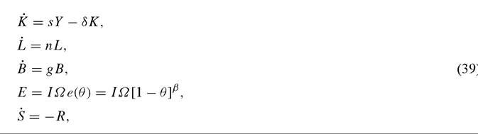
With these assumptions in hand, the production side of the economy becomes
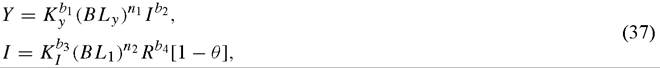
where I is the energy intermediate, θ is the fraction of the energy industry’s activities devoted to abating pollution, R denotes the flow of resources used per unit time, and subscripts denote quantities of capital and labor used in final good production Y, and the intermediate good energy I.
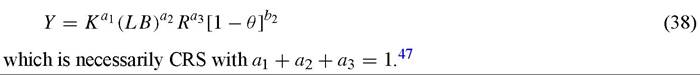
Capital and labor has to be allocated efficiently across the two activities - intermediate and final good production. It is straightforward to show that this implies a constant fraction of the capital stock is employed in intermediate good production and the remainder in final goods. The same is true for labor. This allows us to aggregate and rewrite the production function for final good output as follows
To complete the model we add equations governing the labor force and technology growth, the relationship between extraction and the resource stock S, plus our abatement assumptions linking emissions to energy use I. These conditions are:
 ) where e(θ) measures the flow of emissions released per unit of energy used. It is instructive at this point to rewrite the emissions equation to focus on the role of a changing composition of inputs in determining pollution levels. To do so define the variable χ = I/Y which is the ratio of energy use to final good production, or what is commonly called the energy intensity of GDP. Then rewriting the emissions function we find

A change in emissions can now come from any one of three sources: scale effects via changes in final good output Y; composition effects coming from changes in the energy intensity of final good production χ; and technique effects that lower e(θ) directly.
We examine balanced growth paths and impose two requirements on the set of paths we investigate. First, as usual we require nondeteriorating environmental quality. Second, we require positive growth in per capita income.[511] [512]
To solve for a balanced growth path note Y/K must be constant along any such path. Using this requirement we can log differentiate (38) with respect to time, impose the requirement that Y/K be constant, and find the growth rate of final output49

The first term is the usual growth rate of output in the Solow model; the second is a negative element capturing the growth drag caused by natural resources. To see why this term appears suppose resources were in unlimited supply; then their services could grow over time at the same rate as effective labor and we would have gR = g + n. In this case, capital, output, resources and effective labor would grow at the rate g + n and there would be no resource drag. In fact, however, the resource base 5(0) > 0 is finite and exhaustible, and this implies that gR < 0.50 Any nonpositive gR is feasible because we can always choose the level of resource use such that the finite stock is eliminated asymptotically. Therefore, the ratio of resources to effective labor in production falls over time and this reduces growth below the Solow level. Indeed as (41) shows, growth in final output could be negative if resource constraints loom too large.51
From our earlier equations it is straightforward to show that a3 = b2b4 and hence the existence of finite resources lowers growth by an extent determined by the resource share in final output. To see this note that if the share of final output going to resources approached zero, then α3 approaches zero, and Gy in (41) approaches g + n the Solow growth rate.
It is now straightforward to write growth in per capita output as just

which shows technological progress has to offset both population growth and the reduction in resources over time in order for per capita income to rise. To make this clear and relate our model here to the Stokey Alternative, suppose the resource in question offered an indestructible flow of services per unit time; i.e. suppose it was Ricardian land. Then gR = 0 and growth in per capita income is positive if and only if

The left-hand side of (43) represents the Solow forces of technological progress the strength of which depends on the share of labor in overall production and the rate of labor augmenting technological progress. Aligned against these are the Malthusian forces lowering output per person by applying more and more labor to the fixed stock of land. The rate of population growth and the share of land in production determine the strength 
of the Malthusianforces. Note the similarity between (43) and our earlier (30). The condition in (43) arises when gR = 0 and gy > 0; the condition in (30) has gE = 0 and gy > 0. Note the parallel between emissions and resources.
To generate falling pollution we will need a strong compositional shift and hence gR < 0 is our standard case with our first condition for sustainability given by (42). Our second condition is that pollution must fall over time. Log differentiating our emissions function in (39) yields

To eliminate the possibility of emissions falling because of technological progress in abatement as in the Green Solow model, we set gA to zero. To eliminate the possibility of greater abatement efforts holding pollution in check as in the Stokey Alternative, we set ge(θ) = 0. This leaves only changes in the composition of inputs to offset the rising scale effect of ongoing growth.
Straightforward calculations then show that the growth rate of energy per unit of final output is simply given by

The sign of (45) depends on the large bracketed term which given our correspondences given in footnote 36, is negative. Not surprisingly, the energy intensity of final output must fall over time.
Putting the growth rate of output and energy intensity together we find emissions will fall if and only if

Note the first element in (46), (g + n), is exactly the scale effect of output growth in the Green Solow model. And instead of technological progress in abatement appearing to offset the scale effect of growth, we now have emissions per unit of final output falling from the composition effect given by the second negative term. The growth rate of output is lowered by the drag of natural resources and hence as the economy “abates” by altering its input mix this creates drag much as in Stokey (1998).
There is a tension therefore between the desirability of moving away from natural resource use in order to lower pollution emissions and the cost of doing so in terms of growth. This of course is a primary concern of many developing countries and has limited their participation in the Kyoto Protocol to limit global warming. Because of our addition of a fixed natural resource, in some cases, composition effects alone cannot generate positive balanced growth with a nondeteriorating environment.
To investigate we graph Gy from (42) and Ge from (46) in Figure 10. We have graphed these growth rates against the rate of change in effective labor per unit resource, that is against [(g + n) - gR], since this term plays a key role in both emissions growth and per capita growth. There are several things to note about it. First, suppose resources
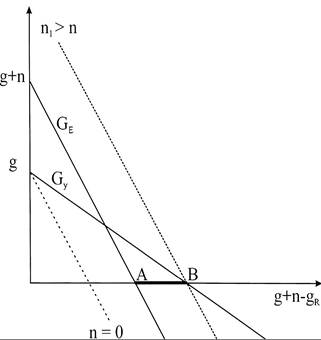
Figure 10. Feasibility: resource drag and per capita growth.
were in unlimited supply; then their services could “grow” over time at the same rate as effective labor g + n. Such a wonderful existence corresponds to points along the vertical axis in the figure. In particular we see that with no resource drag, per capita output growth equals g. With a finite resource base the growth rate of resource use must be negative and this means that per capita income growth must be lower as shown by the negatively sloped line labeled Gy starting at g and intersecting the horizontal axis at point B. Movements along this line correspond to changes in the growth rate of resource use gR.
Similarly, if there were unlimited resources the energy intensity of GDP would remain constant and emissions would rise lock step with output. This unlimited resources scenario corresponds to a point along the vertical axis with the rate of aggregate output growth and emissions of n + g. Again, since resource use must decline over time the true growth rate of emissions must be lower as shown by the line labeled Ge that intersects the horizontal axis at A. The growth rate of emissions falls as we move to the right along this line because final output grows more slowly, and final output uses less energy per unit output.
From these observations it is clear that at all points to the left of A, growth in emissions is positive; points to the right of A, growth in emissions is negative. Similarly, all points to the left of B have positive per capita output growth; points to the right have negative growth. Putting these results together we see that ongoing growth in per capita incomes and an improving environment may not be feasible in some cases. In particular, the bold line segment AB represents the feasible region. Taking g and n as exogenous, this region gives us a range of resource exploitation rates, gR, that are consistent with our twin goals.[513]
To understand the determinants of the feasible region it proves useful to consider the zero population growth case. If population growth is zero, then the two lines have the same vertical intercept as shown by the dotted n = 0 line that is parallel to Ge. Whether positive growth and falling emissions is possible only depends on the relative slopes of Ge versus Gy. Algebra tells us a region such as AB will always exist with zero population growth. The logic is simply that emissions growth falls with both reduced output growth and a changing energy intensity of production. Both occur as we increase drag by moving right in the figure. Therefore, once resource drag has lowered per capita output growth to zero at a point like B the scale effect is zero, but emissions growth must be strictly negative because the composition effect is still driving energy intensity downwards. Consequently, a feasible region like AB exists.
When population growth is positive, this logic fails. As we raise the population growth rate the Ge curve shifts to the right and eventually intersects the horizontal axis at B. This in effect raises the scale effect. At this point, positive growth with declining emissions is not possible. The reason is simply that emissions growth is rising in n (a scale effect), whereas growth in output per capita relies falls with n because of resource drag. Once we choose n large enough - as shown by the dashed line labeled n1 > n - the feasible region disappears.[514]
These results have a decidedly negative flavor to them. An environmental policy that lowers the growth rate of emissions and lowers the energy intensity of final output, also lowers per capita growth to such an extent that an improving environment and real income gains may be unattainable. There are several reasons why we should be cautious in interpreting these negative results. The first is simply that we have ruled out a role for active abatement as in the Stokey Alternative. And we have ruled out technological progress as in the Green Solow model. While adding more avenues of adjustment is always good, active abatement lowers pollution emissions but creates drag just as reducing energy use does. Routine calculations show that if we let all three avenues of adjustment operate, we can write our two balanced growth path requirements as
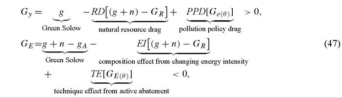
where RD is a positive constant representing resource drag, and PPD a positive constant representing pollution policy drag. Note that in general with both resource exhaustion
and abatement rising, there are two sources of drag on per capita income growth. Corresponding to each source of drag is of course a component of emission reduction. In the second equation EI is a positive coefficient representing energy intensity changes. This corresponds to a composition effect. In addition TE is a positive coefficient representing changes coming from increased abatement; this represents a technique effect.
Putting all this together in terms of our figure, we find that allowing for technological progress in abatement shifts the growth of emissions line G e inward expanding the feasible region. This should come as no surprise. Adding active abatement shifts both lines down (the economy grows slower as do emissions), having an ambiguous effect on the feasible region. Raising population growth from zero however shrinks the region making it more likely that both requirements cannot be met.
What then are we to make of our stylized facts from the introduction? Emission levels have been falling in many countries while growth in per capita income remained positive. Pollution abatement costs have trended upwards but only slowly, and energy prices - while rising - have not been rising at fast rates.[515] We have already seen that these features are roughly consistent with the Green Solow model, but less so with the Stokey Alternative. Here we find that relying on changes in energy intensity alone can work in lowering emissions but it does so only with strong compositional shifts towards less energy intensive goods. In our formulation these shifts are only consistent with a rising real price of energy over time. To see this note that energy’s share in final output is fixed; take final output as the numeraire, and conclude that the real price of energy must rise along the balanced growth path at the rate -/ > 0.
In Figure 11 we plot the real price of three energy sources: oil, natural gas, and coal. For ease of reading all prices are set to 100 in 1957. It is very risky to draw any strong conclusions from this data. The real price of oil has almost doubled since 1957; the price of natural gas is rising quite quickly, while the price of coal has increased the least over the period. Naturally these price increases have created some composition effects as predicted by our source and sink model, but only over certain periods of time. For example, Sue Wing and Eckhaus (2003) examine the history of energy intensity in U.S. production and divide its changes into those accruing from a changing mix of U.S. industries and those accruing from within industry improvements in energy efficiency (which would correspond to a fall in Ω). Their findings suggest that from the late 1950s until the mid-1970s changes in the composition of U.S. industries played a major role in reducing overall energy intensity. But during the 1980s and 1990s the reduction in U.S. aggregate energy intensity has come from improvements in energy efficiency at the industry level. Therefore changes in the composition of output cannot carry the burden of explanation of our data.
Instead these compositional changes must have been helped along by significant technological progress in abatement or energy efficiency (Ω). The evidence for these
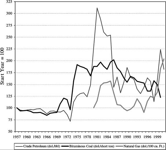
Figure 11. Realenergyprices.
changes is very strong. For example in a detailed study of the energy efficiency of consumer durables Newell, Jaffe and Stavins (1999) find strong support for a significant role for autonomous technological progress (over 60% of the change in energy efficiency), and supporting roles for induced innovation created by higher energy prices. Similar evidence is presented by Popp (2002) who examines the impact of higher energy prices on the rate of innovation in key energy technologies. Usingadatabase of U.S. patenting activity over the 1970-1993 period, Popp explains variation in the intensity of energy patenting across technology groups as a function of energy prices, the existing “knowledge stock” in a technology area and other covariates such as federal funding for R&D. There are two main results from the study. The first is that a rise in energy prices shown in Figure 11 created induced innovation and a burst in patenting activity after the oil price shocks.
The second major result is that while prices are a significant determinant of patenting activity, other factors are also very important. For example, the existing stock of knowledge (as measured by an index of previous patenting weighted for impact) in a technology area has a large impact on subsequent patenting. For example, Popp reports that the average change in knowledge stocks over the period raise patenting activity on average by 24%; while the average change in energy prices over the period raise patenting on average by only 2%. Knowledge accumulation and spillovers are very important in determining the pace of future innovation.[516]
Taking these considerations into account would likely expand our feasible region AB. For example, if the emission intensity Ω fell when either energy prices rose (as in the source-and-sink model) or abatement intensified (as in the Stokey Alternative), then composition changes and active abatement could play a smaller role in checking the growth of pollution. This would of course make feasibility more likely.
Adding complications to our existing models would however take us too far afield, and as yet we know of no research that explicitly links energy prices, induced innovation and pollution emissions within a growth framework. Instead we take a small step towards a theory of induced innovation in the next section when we introduce a model with learning by doing in abatement and reconsider our stylized facts. But before doing so, we should note that we have, to a certain extent, stacked the decks against sustainable growth by assuming environmental quality has no effect on production possibilities. We have assumed that reducing the flow of emissions has only a cost in terms of drag and no benefit in terms of heightened productivity in goods production due to higher environmental quality. Several authors have however postulated a direct and positive link between the productivity of final goods output and environmental quality. This link casts doubt on the validity of growth drag exercises like ours. A typical formulation would add to our models a shift term on the final goods production function that is increasing in environmental quality. For example, Bovenberg and Smulders (1995) and Tahvonen and Kuuluvainen (1991) both postulate this type of additional interaction. Once we allow for a direct productivity response to an improved environment it is not clear that emission reductions lower growth. Bovenberg and Smulders, and Tahvenen both give sufficient conditions under which this additional channel dominates.
In general the less important are emissions in the direct production function, the more responsive is natural growth to a reduction in emissions, and the greater is the marginal productivity boost from a cleaner environment, the more likely it is that these secondary effects will dominate. While it is certainly plausible that a deteriorating environment will lower productivity, it is however unclear how important these impacts are empirically. We suspect that for most of industrial production these environmental impacts are small, or at least fairly elastic over the current range of exploitation. Certain industries such as farming or fishing are certain to have larger productivity effects from an improved environment, but these industries are small contributors to GDP in developed countries. It is likely that these induced productivity effects are greatest in poor developing economies and as yet have escaped the notice of serious empirical researchers.
While it is certainly possible for these direct productivity effects to exist, we feel the biggest restriction imposed by our analysis thus far is its failure to link the rising costs of pollution control to innovation targeted at raising the productivity of abatement. Induced changes in technology of this sort are likely to lower energy intensity over time given the price paths shown in Figure 11; and induced innovation in abatement technologies are likely to be forthcoming as abatement costs rise. Both of these induced effects would lower emissions per unit final output by altering Ω. There is of course a large body of empirical research finding just such effects. But clearly these links are important although difficult to model in a growth framework, for as Popp notes:
The most significant result [sic of the study] is the strong, positive impact energy prices have on new innovations. This finding suggests that environmental taxes and regulations not only reduce pollution by shifting behavior away from polluting activities but also encourage the development of new technologies that make pollution control less costly in the long run... simply relying on technological change is not enough. There must be some mechanism in place that encourages new innovation (p. 178).
With this quote in mind we now turn to consider the impact of technological progress spurred on by the introduction of regulation.
5.