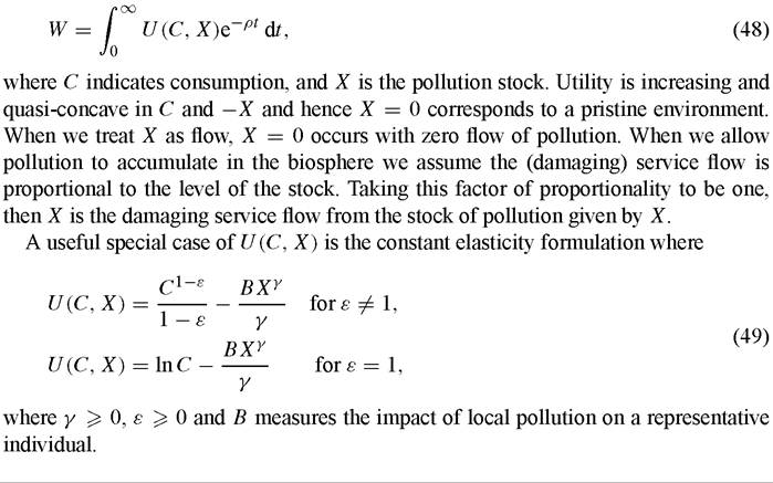
Induced innovation and learning by doing

The series of models we have examined thus far explain the growth and environment history by focusing on technological progress in goods production, increased abate­ment efforts or changes in the composition of output over time.^[517] Missing from this list is a consideration of induced innovation lowering abatement costs.

The possibility of learning by doing offers several new features to the growth and environment relationship. First, if abatement efforts are subject to learning by doing then this feature alone may generate the prediction of a first worsening and then improving environment. In a static setting, learning by doing is identical to increasing returns, and Andreoni and Levinson (2001) show how increasing returns to abatement can generate an EKC in a partial equilibrium endowment economy.^[518]

Secondly, learning by doing alters the costs of pollution control. If learning by doing effects are unbounded, then growth with falling pollution levels could conceivably come at decreasing cost to society. In a world with bounded learning by doing the implications are less clear, but it seems likely that the drag of pollution policy may be smaller if learn­ing by doing effects are present.

Third, if learning by doing arises from economy wide growth in the knowledge stock then learning by doing models offer the possibility of linking technological progress in abatement with that in goods production. As our previous analysis makes clear the relative rates of technological progress in goods production and abatement are key to determining the sustainability of a balanced growth path. This was especially clear in the Green Solow model, but was implicit in the other formulations because the absence of technological progress in abatement required other compensating changes to hold pollution in check. Learning by doing models give us one way to make our assumptions about knowledge spillovers and technological progress consistent across sectors.

Finally, although learning by doing is often modeled as a passive activity and not purposeful investment, learning by doing can be a form of induced innovation. If a worsening environment necessitates the imposition of pollution controls, and abatement is subject to learning by doing, we have effectively followed the advice of Popp in identifying a causal factor behind subsequent improvements in abatement technology.

5.1. Induced innovation and the Kindergarten Rule model

To discuss these issues, we now introduce the Kindergarten Rule model of Brock and Taylor (2003). This model, like those in the static literature, relies on learning by doing in the abatement process to hold pollution in check. Importantly, though since learning by doing is really an assumption about knowledge spillovers, the Kindergarten model adopts a consistent set of assumptions regarding the beneficial impact of knowledge spillovers.

In order to focus on the implications of ongoing technological progress for the envi­ronment and growth, Brock and Taylor (2003) adopt the very direct link between factor accumulation and technological progress employed by Romer (1986), Lucas (1998) and others. By doing so they generate a simple one-sector model of endogenous growth and environmental quality. But as is well known, one-sector models of endogenous growth blur the important distinction between physical capital and knowledge capital and force us to think of “capital” in very broad terms.⁵⁸

For simplicity they adopt a conventional infinitely lived representative agent, and assume all pollution is local. There is one aggregate good, labeled Y, which is either consumed or used for investment or abatement. There are two factors of production: labor and capital. There is zero population growth and hence L(t) = L; recall it is the rate of population growth relative to the rate of technological progress that is key, so here one of these rates is set to zero. In contrast to labor, the capital stock accumulates via investment and depreciates at the constant rate δ.

5.1.1. Tastes

A representative consumer maximizes lifetime utility given by:

^[1] Extensions of their framework to allow for purposeful innovation and a distinction between these two forms of capital, along the lines of Grossman and Helpman (1991) or Aghion and Howitt (1998), seem both feasible and worthwhile.

5.1.2. Technologies

The assumptions on production are standard. Each firm has access to a strictly concave and CRS production function linking labor and capital to output Y. The productivity of labor is augmented by a technology parameter T taken as given by individual agents. Following Romer (1986) and Lucas (1998) we assume the state of technology is propor­tional to an economy wide measure of activity. In Romer (1986) this aggregate measure is aggregate R&D, in Lucas (1998) it is average human capital levels; in AK specifi­cations it is linked to either the aggregate capital stock or (to eliminate scale effects) average capital per worker. We assume T is proportional to the aggregate capital to la­bor ratio in the economy, K∕L, and by choice of units take the proportionality constant to be one.^[519]

5.1.3. From individual to aggregate production

Although we adopt a social planning perspective, it is instructive to review how firm level magnitudes aggregate to economy wide measures since this makes clear the as­sumptions made regarding the role of knowledge spillovers. We aggregate across firms to obtain the AK aggregate production function as follows:^[520]

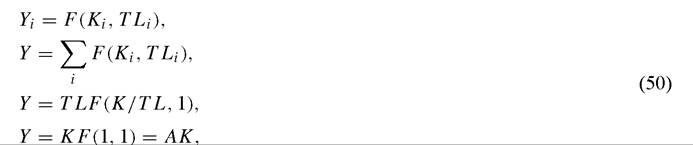
where the first line gives firm level production; the second line sums across firms; the third uses linear homogeneity and exploits the fact that efficiency requires all firms adopt the same capital intensity. The last line follows from the definition of T.

Summarizing: diminishing returns at the firm level are undone by technological progress linked to aggregate capital intensity leaving the social marginal product of capital constant.

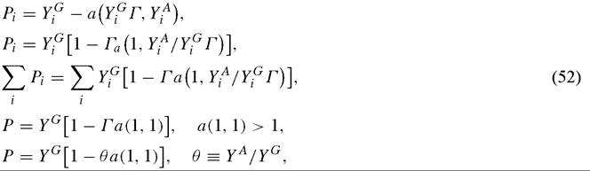
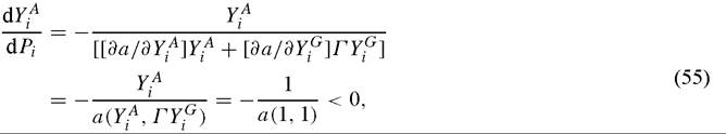
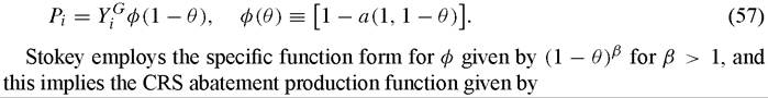
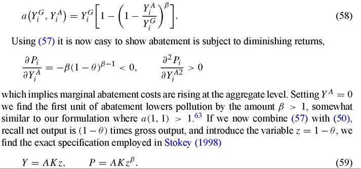
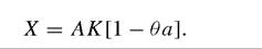
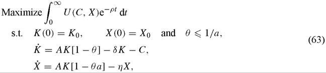
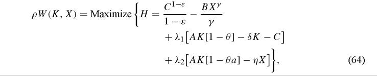
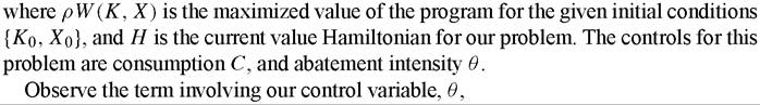
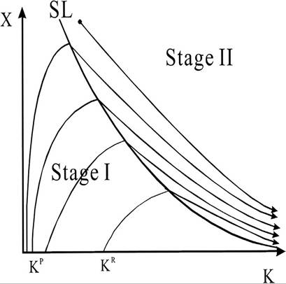
We now employ similar methods to generate the aggregate abatement technology. To start we note pollution is a joint product of output and we take this relationship to be proportional.^{[521] [522] By choice of units we take the factor of proportionality to be one.}

Now consider a Romeresque approach where individual abatement efforts provide knowledge spillovers useful to others abating in the economy. To do so we again in­troduce a technology shift parameter Γ, and assume it raises the marginal product of abatement. To be consistent with our earlier treatment of technological progress in pro­duction we assume Γ is proportional to the average abatement intensity in the economy, Y^a∕Y^g. Then much as before we have the individual to aggregate abatement technol­ogy transformation as

given by foregone output used in abatement, and hence partially differentiating the sec­ond line of (52) and rearranging we find

Marginal abatement costs are rising at the firm level.

Marginal abatement costs at the society level, are however, constant. To see why totally differentiate (52) allowing Γ and individual abatement to both vary. We find

Γ is the average abatement intensity in the economy, which given identical firms, is just the abatement intensity for the typical ith firm. Using = [1/Y_i^G][dY_i^A/dP_i] and rearranging (54) we obtain

where the first line follows from rearrangement and the second by CRS in abatement.

Summarizing: diminishing returns at the firm level, that lead to rising marginal abatement costs, are undone by technological progress linked to aggregate abatement intensity leaving the social marginal cost of abatement constant.

The formulations of learning by doing that we have adopted are extreme. In gen­eral we would expect the productivity in abatement (or production) to adjust gradually in response to a slow moving measure of knowledge capital. In the cases developed here however the productivity boost from an increased knowledge capital occurs instan­taneously. So instead of Γ being a complicated function of the abatement intensities adopted in the infinite past history of the economy weighed by their relevance to pro­ductivity today, it is simply proportional to the current intensity. This is of course an abstraction, but a useful one since it frees us from keeping track of the evolution of two additional state variables (knowledge capital in abatement and knowledge capital in production), and allow us to capture the main feature of learning by doing models by linking the productivity of abatement to the intensity of this activity at the econ­omy wide level. It also yields simple linear forms for production and abatement that add greatly to the model’s tractability. This last features is especially important in a model where the stock of environmental quality has already raised the number of state variables to two.

Putting these pieces together our planner faces the aggregate production relations for output and abatement given by the last lines of (50) and (52) together with the atemporal resource constraint linking gross output, abatement and net production

The Kindergarten model is only one approach to modeling endogenous growth and environment interactions. Closely related approaches in an AK framework are those of Stokey (1998), Smulders (1994) and Smulders and Gradus (1996). These papers all adopt AK models, but end up with different conclusions. Early work in a one-sector framework by Smulders (1994) and Smulders and Gradus (1996) demonstrated how continuing economic growth and constant environmental quality are compatible in an AK model. In contrast, Stokey (1998) demonstrated how continuing growth and con­stant environmental quality are not possible within an AK set-up. The difference in their results comes from their different assumptions on abatement. To see why this is true, start with (51), ignore knowledge spillovers, and work forward using now familiar steps to find:

Stokey’s (1998) result that growth is not possible follows from matching an AK aggregate production function with strictly n eoclassical assumptions on abatement adopted from Copeland and Taylor (1994). That is, if we think of the AK model as one of knowledge spillovers then Stokey has assumed these spillovers occur in production but not abatement. By doing so, she eliminates “technological progress” in abatement and this eliminates the possibility of sustainable growth.

⁶³ Since the marginal product of abatement is bounded at zero, Stokey (1998) shows no regulation is under­taken initially and pollution rises lock-step with output.

Comparing our approach to the work of Smulders is more difficult because abatement is not specifically modeled and he considers a variety of formulations. By specializing his framework to the AK paradigm we find

The first element is just a standard AK production function. The second relates what Smulders refers to as net or emitted pollution to the capital stock K, and abatement A. If we employ (60) and solve for emissions per unit of gross output we find

If the economy allocates a fixed fraction of its output to abatement, K/A is con­stant, and emissions per unit of gross output fall with the size of the economy. This reflects a strong degree of increasing returns. Moreover, the reader may note from (60) that pollution emitted goes to infinity as abatement goes to zero, which is inconsistent with pollution being a joint product of output. Therefore, Smulders and Gradus (1996) match AK aggregate production with assumptions on abatement ensuring increasing returns; and, in contrast with the Kindergarten specification, assume pollution is not a joint product of output.

5.1.4. Endowments

We treat pollution as a flow that either dissipates instantaneously - such as noise pollu­tion - or a stock that is only eliminated over time by natural regeneration - such as lead emissions or radioactive waste. When X is a stock we have

where η represents the speed of natural regeneration, and where for economy of notation we have denoted a(1, 1) by a. When X is a flow we have

5.1.5. The Kindergarten rule

We focus first on the possibility of balanced and continual growth, leaving to the next section a discussion of transition paths. Before we proceed with the formal analysis it proves instructive to step back slightly to consider the feasibility and optimality of sustainable growth. From our assumptions on abatement it is clear that if θ is set high enough all pollution emissions will be eliminated and we will enter a zero emission world. Therefore as long as a > 1 there will exist a θ < 1 that generates zero emis­sion technologies. And if θ < 1 then some output will be left over for consumption and investment which will in turn drive growth in output. It appears then that feasibil­ity is guaranteed by knowledge spillovers in abatement generating a constant marginal product.

The assumption of a > 1 is innocuous. Recall that abatement, like all other economic activities, pollutes. One unit of abatement creates one unit of pollution, but cleans up a > 1 units of pollution. It is only this surplus between costs and benefits, 1 - 1/a > 0 that makes abatement useful at all! But even if growth is feasible, abatement is costly and this will cause drag as in our earlier formulations. The remaining questions for sustainability are how large is this drag, how much will it lower the return to capital, and what restrictions on preferences will be needed to generate sustainable growth.

To answer these questions consider the following problem:

where we adopt U(C, X) from (49). Recall the fraction of gross output allocated to abatement is θ and since the flow of pollution into the environment cannot be negative this will never exceed 1/a. We can write the Hamilton-Jacobi-Bellman equation as

of S determines when and if the economy switches from a zero-to-active-to-maximal abatement regime. We deal with these possibilities in turn.

Regardless of the value of S, the optimal level of consumption will always satisfy

In this situation pollution is not completely abated, and hence the evolution of envi­ronmental quality reflects both the level of active abatement and natural regeneration. And finally, with no abatement at all we must have S < 0. Both pollution and output ⁶⁴ This is one of the most common rules taught in Kindergarten. For a list of common Kindergarten rules see All I Really Need to Know I Learned in Kindergarten: Uncommon Thoughts on Common Things by Robert Fulgham. Fulgham argues that the basic values we learned in grade school such as “clean up your own mess” (in effect our Kindergarten rule) and “play fair” are the bedrock of a meaningful life.

Consider growth paths with active abatement. Then from (67) and (66) we find the shadow value of capital falls over time at a constant exponential rate,

)

provided the net marginal product of capital, at the Kindergarten rule level of abatement, A[1 - θ_κ], can cover both depreciation and impatience. We leave for now a detailed discussion of what this requires and assume it is true: g > 0. Then it is immediate that consumption rises at the constant rate g_c = g∕ε > 0.

From the capital accumulation equations in both (66) and (67) we can now deduce that capital and output must grow at the same rate as consumption if θ is constant over time. To determine whether the intensity of abatement is constant over time, consider the accumulation equation for pollution

There are two ways (70) can be consistent with balanced growth. The first possibility is that we have a maximal abatement regime where S > 0 holds everywhere along the balanced growth path. In this situation, K grows exponentially over time and θ is set to the Kindergarten rule level. Using (66), this balanced growth path must have

In this scenario, the environment improves at the rate η over time and abatement is a constant fraction of output 1 > θ_κ > 0. As time goes to infinity the economy approaches a pristine level of environmental quality. Therefore the balanced growth path exhibits constant growth in consumption, output, capital and environmental quality. Consumption is a constant fraction of output and we have

A second possibility is that abatement is active but not maximal. Define the deviation of abatement from the Kindergarten rule as D(θ) = (θ_κ — θ )∕θ_κ. Using this definition rewrite (70) to find

It is apparent that if the deviation of abatement from the Kindergarten rule fell expo­nentially, then it may be possible for X to fall exponentially while K rises. That is, in obvious notation, a possible balanced growth path would have

In this situation abatement is at an interior solution at all times and becomes progres­sively tighter over time approaching the Kindergarten rule asymptotically. The inflow of pollution from production into the environment is always positive but environmental quality improves nevertheless. This intuitive description suggests that the possibility of this outcome must rely on both the pace of economic growth and the ability of the en­vironment to regenerate. This is indeed the case as Brock and Taylor (2003) show that a necessary condition for us to remain in an S = 0 regime is simply

This condition reflects two different requirements. The first is simply that γ cannot equal one. If it did then the (instantaneous) marginal disutility of pollution is a constant and λ₂ is a constant as well. This would also imply that consumption be fixed as well. This is inconsistent with growth of any sort.

Assuming γ not equal to one is necessary for balanced growth with an interior so­lution for abatement. But a second condition must also hold. Natural regeneration, η, must be sufficiently large relative to the growth rate g. If the rate of regeneration is high and growth rates quite low, then the optimal plan is to use nature’s regenerative abilities to partially offset the costs of abating because the shadow value of foregone output is high in slow growth situations. Conversely, if regeneration is low and the growth rate g relatively high, then no amount of abatement short of the Kindergarten rule will hold pollution to acceptable levels.

This intuition suggests a natural corollary for the case of flow pollutants. If pollution has only a flow cost it is “as if” the environment is regenerating itself infinitely fast. This intuition suggests that as we let η get large, the results in the stock pollutant case should replicate those for a flow. This intuition is, in fact, correct. Brock and Taylor prove that when g > 0 and X is a flow pollutant, then sustainable economic growth with an ever improving environment is possible and optimal. With a flow pollutant, if γ > 1, then the intensity of abatement approaches the Kindergarten rule level of abatement, θ_κ, asymptotically. Alternatively, if γ = 1, then θ = θ_κ everywhere along the balanced growth path.

These results are important in showing how the Kindergarten rule generates sustain­able growth. Sustainable growth requires two conditions. The first is that g > 0. The assumption g > 0 requires the marginal product of capital, adjusted for the ongoing costs of abatement, be sufficiently high. A necessary condition is that A[1 - θ_κ] be posi­tive, but this is guaranteed as long as abatement is a productive activity. Given abatement is productive, we still require the adjusted marginal product of capital, A[1 - θ_κ], to off­set both impatience and depreciation. If abatement is not very productive, then 1 /a will be close to one and growth cannot occur. If capital is not very productive or if the level

of impatience and depreciation are high then ongoing economic growth cannot occur. These are however very standard requirements for growth under any circumstances; therefore our addition of the further requirement that abatement be productive seems both innocuous and natural in our setting.^[523]

The second is that h = g(1 - 1∕ε) + p > 0. This condition is the standard sufficiency condition for the existence of an optimum path in an AK model with power utility.^[524] This condition is of course weaker than that needed in earlier models generating declin­ing pollution levels. For example, ε is just σ in the CRRA specification we used earlier and we have already seen that Stokey (1998), Lopez (1994) and other require σ > 1 to generate declining emissions. Here the requirement is far weaker and this follows from the fact that consumer’s are not required to make larger and larger sacrifices in consumption to fund an every growing abatement program.

5.2. Empirical implications

The Kindergarten model relies heavily on the assumed role of technological progress in staving off diminishing returns to both capital formation and abatement. It is impossible to know a priori whether technological progress can indeed be so successful and hence it is important to distinguish between two types of predictions before proceeding. The first class of predictions are those regarding behavior at or near the balanced growth path. This set has received little attention in the empirical literature on the environment and growth, although balanced growth path predictions and their testing are at the core of empirical research in growth theory proper [see the review by Durlauf and Quah (1999)]. The second set of predictions concern the transition from inactive to active abatement and these are related to the empirical work on the Environmental Kuznets Curve. [See Grossman and Krueger (1993, 1995) and the review by Barbier (1997).]

5.3. Balanced growth path predictions

Using our previous results it is straightforward to show that near the balanced growth path we must have: convergence in the quality of the environment across all countries sharing parameter values but differing in initial conditions; the share of pollution abate­ment costs in output approaching a positive constant less than one; overall emissions rates falling and environmental quality rising; and emissions per unit output falling as production processes adopt methods that approach zero emission technologies. The model also presents predictions for the intensity of abatement that we discuss subse­quently.

Whether the cross-country predictions will be borne out by empirical work is as yet unknown but an examination of U.S. data shows the model’s strongest predictions - those regarding falling emissions and improving environmental quality - are not grossly at odds with available U.S. data. The most favorable evidence for the model is the slow movement in pollution abatement costs in the face of dramatically declining pol­lution levels. The model explains this feature of the data by recourse to specifics of the abatement function that hold abatement costs down much as exogenous technological progress does in the Green Solow model.

The prediction of declining emission intensities along the balanced growth path is consistent with the data shown in Figure 1, but as in Stokey (1998) the model only predicts declining emissions to output ratios after regulation begins.

5.4. The Environmental Catch-up Hypothesis

We have so far focused on balanced growth paths but the large EKC literature con­cerns itself with what must be transition paths towards some BGP. To examine these predictions and these always exhibited active abatement. It is however natural to ask predictions we present several transition paths in Figure 12. One of these paths is that of a Poor country having small initial capital K^p but a pristine environment. The other is the path of a Rich country starting again with a pristine environment but with a much larger initial capital K^r. Each economy starts with a pristine environment in Stage I and grows. During this stage there is no pollution regulation: the environment deterio­rates, X rises, and the capital stock grows until the trajectory hits the Switching Locus labeled SL. Once the economy hits the Switching Locus active regulation begins and the economy enters Stage II.6⁷

It is apparent from the figure that the Poor country experiences the greatest environ­mental degradation at its peak, and at any given capital stock, (i.e. income level) the initially Poor country has worse environmental quality than the Rich. Moreover, since both Rich and Poor economies start with pristine environments, the qualities of their environments at first diverge and then converge. This is the Environmental Catch-up Hypothesis.

Divergence occurs because the opportunity cost of abatement (and consumption) is much higher in capital poor countries. A high shadow price of capital leads to less

⁶⁷ Brock and Taylor (2003) show the exact position and shape of the locus depend on whether parameters satisfy the fast growth or slow growth scenario. For the most part we will proceed under the assumption that economic growth is fast relative to environmental regeneration; that is (75) fails strongly and we have η(γ — 1) > g. This implies θ(t) = θκ everywhere along the balanced growth path (Figure 12 implicitly assumes this result). For illustrative purposes we will sometimes discuss the parallel flow case [where we can think of η approaching infinity but (75) failing because γ = 1].

Figure 12. Transition paths.

consumption, more investment and rapid industrialization in the Poor country. Nature’s ability to regenerate is overwhelmed. The quality of the environment falls precipitously. In capital rich countries the opportunity cost of capital is lower: consumption is greater and investment less. Industrialization is less rapid and natural regeneration has time to work. The peak level of environmental degradation in the Rich country is therefore much smaller. But once we enter Stage II abatement is undertaken and since abatement is an investment in improving the environment, it is only undertaken when the rate of return on this investment equals (or exceeds) the rate of return on capital. Since economies are identical, except for initial conditions, rates of return are the same across all countries in Stage II. Equalized rates of return require equal percentage reductions in the pollution stock. Therefore absolute differences in environmental quality present at the beginning of Stage II disappear over time.

Note how similar this intuition for the ECH is to that given for the EKC prediction in the Green Solow model. In the Green Solow model initially rapid growth overwhelms nature’s ability to dissipate pollution starting from its initial position at a biological equilibrium. Eventually growth slows and the environment’s regenerative powers re­store its quality slowly over time. Growth is initially rapid in the Solow model because of diminishing returns. In the Kindergarten model, growth is initially rapid because there is no regulation and no drag from pollution policy to lower the marginal product of capital. And once regulation is active, growth slows because regulation lowers the net marginal product of capital. The environment’s regenerative powers then restore its quality slowly over time. Both explanations have nature overwhelmed early on and both give prominent roles to a declining marginal product of capital.

The discussions above, and Figure 12, assume the fast-growth-slow-regeneration as­sumptions hold. We chose this case to discuss and illustrate because it illustrates the forces at work very clearly. Since many of the same conclusions hold when growth is relatively slow we only provide a sketch here of some differences. There is again a Switching Locus which divides Stage I from Stage II. The Switching Locus again de­fines a unique X* that is declining in K*. The most important difference is that once a trajectory of the system hits this new Switching Locus it remains within it forever. If the economy is below the locus then abatement is inactive and K rises at a rapid rate: X in­creases rapidly until the Switching Locus is reached in finite time. If the initial (K, X) is above the locus, maximal abatement is undertaken but this drives down the shadow cost of pollution very quickly and we again hit the locus, this time, from above.

Once on the locus, countries remain trapped within it thereafter and this implies the economy’s choice of abatement remains interior; i.e. the trajectory follows along the Switching Locus maintaining MAC = MD(K, X) throughout. Over time abatement rises and the intensity of abatement approaches the Kindergarten rule in the limit. There­fore, the slow growth case is very similar except that the model now predicts an strong form of convergence. All transition paths remain on the Switching Locus once active abatement begins; therefore policy active countries share the same path for environmen­tal quality and income levels in Stage II.

5.5. The ECH and the EKC

Brock and Taylor prove that economies follow the Stage I-Stage II life cycle pro­ducing an EKC like relationship between income and environmental quality.^[525] Their income and growth prediction is however somewhat different from a standard EKC result. They predict that countries differentiated only by initial capital exhibit initial di­vergence in environmental quality followed by eventual convergence.^[526] Moreover, as Figure 12 makes clear countries make the transition to active abatement at different in­come and peak pollution levels. This of course throws into question empirical methods seeking to estimate a unique income-pollution path. More constructively it suggests that an important feature of the data may well be a large variance in environmental quality at relatively low-income levels with little variance at high incomes. Empirical work by Carson, Jean and McCubbin (1997) relating air toxics to U.S. state income levels is supportive of this conjecture:

Without exception, the high-income states have low per capita emissions while emissions in the lower-income states are highly variable. We believe that this may be the most interesting feature of the data to explore in future work. It suggests that it may be difficult to predict emission levels for countries just starting to enter the phase, where per capita emissions are decreasing with income (pp. 447-448).

In some cases however, (initially) Rich and Poor will make the transition at the same income level but still exhibit our Catch-up Hypothesis. To investigate, we report the switching locus in the fast growth case. It takes on an especially simple form given by which is the downward sloping and convex relationship between pollution and capital depicted in Figure 12. The left-hand side of (76) represents marginal abatement costs. The right-hand side is marginal damage evaluated at {K*, X*}. Marginal damage is increasing in the pollution stock provided γ exceeds one, and since the flow of national (and per capita) income Y is always proportional to K, it is apparent that the income elasticity of marginal damage with respect to flow income is given by ε. Large values of ε correspond to the strong income effects referred to earlier.

Let γ approach one. Then the slope of the Switching Locus approaches infinity and all countries attain their peak pollution levels at the same K*. But even with a com­mon turning point differences in environmental quality remain. Moreover, these are not simple level differences because countries initially diverge and then converge after crossing K*. To eliminate our catch-up hypothesis we must assume regeneration is infi­nitely fast: X is a flow. In this case Brock and Taylor show the Switching Locus is again vertical at a given K *. More importantly, since pollution is proportional to production before K *, and policies are identical after K *: initial conditions no longer matter.

These results tell us that when pollution is strictly a flow, all countries share the same income-pollution path. We have generated an EKC, and empirical methods used to estimate a unique income-pollution path are appropriate. But when pollution does not dissipate instantaneously, initial conditions matter. We have the Environmental Catch­up Hypothesis, and empirical methods must now account for the persistent role of initial conditions.^[527] It is easy to see the two hypotheses are mutually exclusive and exhaustive.

5.6. Pollution characteristics

The ECH focuses on cross-country comparisons in pollution levels, but says little about how predictions vary with pollutant characteristics. And while most authors have fo­cused on generating an EKC relationship there has been very little work examining

how these predictions vary with pollutant characteristics. This is unfortunate since there is good data in the U.S. and elsewhere that could be fruitfully employed to test within country but across pollutant predictions. This is especially important since many models can generate the EKC result.

To demonstrate the Kindergarten model’s across pollutant predictions consider re­generation first and start from a position where η = 0 (radioactive waste). Brock and Taylor (2003) show that the Switching Locus in Figure 12 shifts outwards as we raise η. The response is to delay action and allow the environment to deteriorate further. Once we raise η sufficiently the economy eventually enters the fast regeneration regime and here we find abatement delayed in another manner - it is introduced slowly by the now gradual implementation of the Kindergarten rule. Faster regeneration then implies that countries either begin abatement at higher income levels or allow their environments to deteriorate more before taking action. Surprisingly, fast regeneration will be associated with lower and not higher environmental quality - at least over some periods of time or ranges of income.^[528]

A change in regeneration rates also affects the pace of abatement. If a pollutant has a long life in the environment, then once abatement begins it is clear that natural regenera­tion can play only a small role. Consequently the optimal plan calls for an initial period of inaction before starting a very aggressive abatement regime: the immediate adop­tion of the Kindergarten rule. When η is relatively large we are in the fast regeneration regime and abatement is intensified gradually and only approaches the Kindergarten rule level in the limit.

Putting the predictions for the timing and intensity of abatement together, Brock and Taylor find that very long-lived pollutants should be addressed early with their complete elimination compressed in time. It is optimal to delay action on short-lived pollutants and adopt only a gradual program of abatement. This description of optimal behavior is of course consonant with the historical record in several instances where long-lived chemical discharges and gas emissions were eliminated very quickly by legislation, whereas short-lived criteria pollutants have seen active regulation but not elimination over the last 30 years.

Pollutants also differ in their toxicity. The marginal disutility of toxics could exceed those classified as irritants, and damages from toxics may rise more steeply with ex­posure. The first feature of toxics implies their abatement should come early. This is clear from (76) where increases in B shift the Switching Locus inwards and hasten abatement. Surprisingly very convex marginal damages (a high γ) call for the grad­ual and not aggressive elimination of pollution. The logic is that any reduction in the concentration of toxics has a large impact on marginal damage. Therefore, only by low­ering emissions slowly can we match a steeply declining value of marginal reductions with a falling opportunity cost of abatement. Therefore, although toxics may have large absolute negative impacts on welfare, this argues for their early, but not necessarily aggressive, abatement.

And finally how does the income elasticity of the demand for environmental qual­ity (ε) affects the onset and pace of regulation? We have already shown that the re­striction of ε > 1 is not needed to generate sustainable growth. This parameter does however have a role to play in determining the timing of regulation. To illustrate its role consider the fast growth regime and let the gross marginal product of capital, A, rise. This necessarily raises g and if ε > 1, the Switching Locus shifts in. Abatement is hastened. When ε < 1, abatement is delayed and peak pollution levels shift right.^[529] A similar set of results holds for increases in the productivity of abatement although there is an additional conflicting force. Therefore, in contrast to earlier work Brock and Taylor (2003) finds that the income elasticity of marginal damage has an important role to play in determining the income level at which abatement occurs and the resulting pollution level, but virtually no role in determining if the environment will improve nor its rate of improvement.

6.