Preliminaries
2.1. Scale, composition and technique
We start with some algebra linking emissions of a given pollutant to a measure of economic activity, its composition and the cleanliness of production techniques.
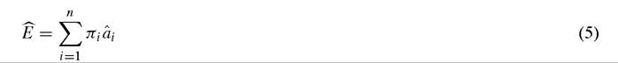
By doing so we illustrate that any growth model that predicts both rising incomes and falling pollution levels has to work on lowering pollution emissions via one of three channels. Consider a given pollutant and let E denote the sum total of this pollutant’s emissions arising from production across the economy’s n industries.[478] Let ai denote the pounds of emissions per dollar of output produced in industry i, si denote the value share of industry i in national output, and Y national output. Then by definition total emissions E are given by
Since this is a definition we can differentiate both sides with respect to time to find

where a over x indicates [dx/dt]/x. Changes in aggregate emissions can arise from three sources that we define to be the scale, composition and technique effects.[479]
To start, note that holding constant the cleanliness of production techniques and the composition of final output constant (i.e. holding both ai = 0 and si = 0 for all i) emissions rise or fall in proportion to the scale of economic activity as measured by real GDP or Y. This is the scale effect of growth and unless it is offset by other changes, emissions rise lock step with increases in real output.
Alternatively, we can hold both the scale of real output and the techniques of production constant to examine the impact of changes in the composition of output. To do so, in (2) we set Y = 0 and ai = 0 for all i as this isolates the pure composition effect on pollution emissions,

Emissions fall via the pure composition effect if an economy moves towards producing a set of goods that are cleaner on average than the set they produced before.
To see why this is true, note that the change in value shares across all n industries must sum to zero; i.e. ∑‰1 dsi = 0. Now using this result in (3) we obtain the change in emissions arising from a pure composition effect as
Given our definitions for π i and si, πi — si > 0 if and only if Ei∕piyi > E /Y.In words, the element πi — si is positive if and only if industry i's emissions per dollar of output is greater than the national average. Define a dirty industry as one whose emissions per dollar of output exceed the economy wide average E/Y; define a clean industry as one where emissions per dollar of output are less than the economy average. Then Equation (4) holds that aggregate emissions fall from the pure composition effect whenever the composition of output changes toward a more heavy reliance on clean industries and rises otherwise.
Finally, emissions can fall when the techniques of production become cleaner even though output and its composition remain constant. To isolate this technique effect, we set Y = 0 and si = 0 for all i to find that emissions fall if emissions per unit output fall for all activities. In this case we find
and hence if techniques are getting cleaner, emissions per unit of output fall, and overall emissions fall from this pure technique effect.
When the environment is modeled as a sink for human wastes it is often assumed that emissions together with natural regeneration determine environmental quality. When the environment adjusts relatively slowly to changes in the pollution level, natural regeneration can play an important role in determining environmental quality. A typical and very useful specification assumes the environment dissipates pollutants at an exponential rate.
Let X denote environmental quality and let the pristine level be given by X = 0. Then since the flow of emissions per unit time is E, the evolution of environmental quality is given by
This formulation is convenient because it is generally assumed that X must be bounded for human life to exist and hence (6) yields a simple negative linear relationship between the steady state flow of pollution E, and environmental quality X. A bound on X then implies a similar bound on steady state emissions, E.[480] Moreover, given the linear relationship any scale, composition or technique effect on emissions is translated directly into impacts on environmental quality, X.
One cost of (6) is that the percentage rate of natural regeneration is independent of the state of the environment. A common modification is to assume the rate of natural regeneration rises as X gets further and further from its pristine level. Letting η = η(X), we can introduce this possibility by writing the evolution of X as

η(X) is often assumed to be linear so that η(X)X becomes the familiar logistic function for growth in X.
An alternative and equally valid interpretation of (2) is that E is the instantaneous flow of natural resources used in production. Under this interpretation, Equation (1) gives us an economy wide factor demand for this natural resource evaluated at the equilibrium level of use given by E. For example, the demand for oil equals the sum of demand arising from all sectors of the economy. In this interpretation ai are barrels of oil used per unit of output in industry i, si is the value share of industry i in national output, and Y is again national output.
For example, if the flow of resources extracted is falling at some constant rate over time while real output is rising, then we know that some combination of changes in energy efficiency per unit of output (a technique effect) and changes in the output mix to less energy intensive goods (a composition effect) must be carrying the burden of adjustment.
Changes in resource use overtime can then be linked to the relative strength of scale, composition and technique effects. To complete the translation let the current stock of natural resources S be given by our initial endowment K less any diminution caused by humans, X. If we make this translation in (6), and set regeneration equal to zero we obtain the standard equation governing stock depletion in exhaustible resources
Alternatively, we can make the same translation but leave open the possibility of regeneration. Making the translation in (7) gives us the standard accumulation equation for a renewable resource such as a forest or fishery when growth is stock dependent,
 i And again if η(S) is linear we obtain the familiar logistic growth for a naturally regenerating resource.[481]
Although (1) is a definition it implicitly contains an assumption on how economic growth and the environment interact. Note that the value shares sum to 1 and ai (t) f 0 for all i and t. Assume that ai(t) for all i and t. This assumption turns out to be an important, because if some activities are perfectly clean, or approach perfectly clean activities in the limit, then it is possible for composition effects alone to hold pollution in check despite ongoing growth. Conversely, if all economic activities must pollute even a small amount, then environmental quality can only rise in the long run via continuous changes in the techniques of production and these may run into diminishing returns.
It is not helpful here to enter into philosophical discussions over the definition of pollution or the likelihood of today’s unwanted outputs becoming tomorrow’s valuable inputs. Instead we just note that all production involves the transformation of one set of materials into another and that this transformation requires work.
All work requires energy and energy is always wasted in work effort. Therefore some unintentional by products of production are always produced and we most often call these by products pollution. Since this is a statement of belief and not a rigorous proof, we note this as an assumption.Assumption 1. Pollution is a by-product of all production

This implies that there exists for each i, a strictly positive ε > 0 such that ai(t) > ε. With Assumption 1 in hand, it is now possible to show that positive output growth and falling pollution levels require falling emissions per unit of output in the long run. That is, composition effects are at best a transitory method to lower pollution emissions. Let us explain in detail why this conclusion holds. Suppose there is a bound, B > 0 such that if E(t) exceeds B, human life cannot exist. Then if Y(t) goes to infinity as t goes to infinity, (10) implies

Thus we must have

But (12) contradicts Assumption 1. Hence if we are to have bounded emissions with growing Y(t), we must have the cleanest industry emission rate ai(t) going to zero. Therefore, falling pollution levels and rising incomes are only possible if there are continual reductions in emissions per unit output and zero emission technologies are possible, at least in the limit.
3. Stylized facts on sources and sinks
We present three stylized facts drawn from post-World War II historical record.[482] We present data on pollution emissions and environmental control costs and leave the discussion of energy prices to later sections. Since data is typically only available for pollutants that are presently under active regulation we discuss the U.S.
record with regard to its six so-called criteria air pollutants, but amend these with international sources where possible. These are: sulfur dioxide, nitrogen oxides, carbon monoxide, lead, large particulates and volatile organic compounds.[483] Withthe exception of lead, these air pollutants all typically classified as irritants and so we also briefly discuss the U.S. history of regulation of long-lived and potentially harmful chemical products. For the most part we present data on emissions rather than concentrations because data on emissions covers a much longer time period and is unaffected by industry location and zoning regulation. On the other hand, the longest time spans of data (from 1940 onwards) reflect some changes in collection and estimation methods.[484] Nevertheless, this data is the best we have available and where possible we direct the reader to concentration data and related empirical work. In addition we present data on industry pollution abatement costs from Vogan (1996), although these are only available for the 1972-1994 period.We start by presenting in Figure 1 emissions per dollar of GDP for all pollutants except lead. Lead is excluded since data is only available over a much shorter period. As shown, emissions per unit of output for sulfur, nitrogen oxides, particulates, volatile organic compounds and carbon monoxide all fall over the 1940-1998 period. For ease of
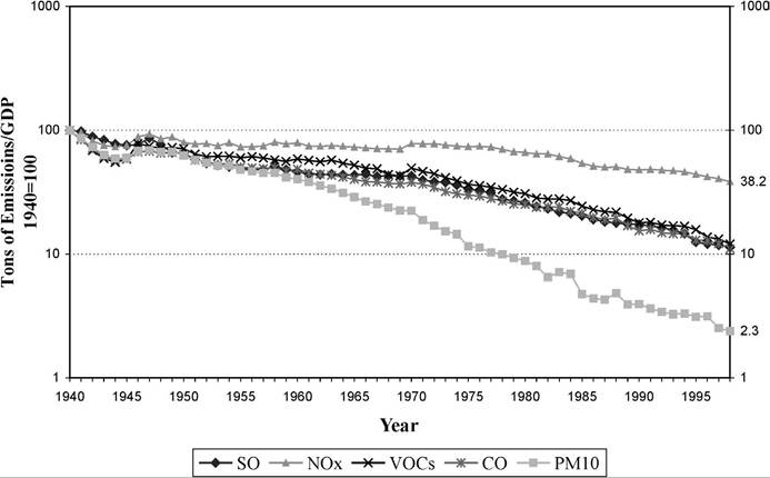
Figure 1. Emission intensities, 1940-1998. Tons of emissions/real GDP.
comparison emission intensities were normalized to 100 in 1940 and the figure adopts a log scale. PM10 fell by approximately 98%, sulfur, volatile organic compounds and carbon monoxide fell by perhaps 88%, and nitrogen oxides fell by perhaps 60%. Somewhat surprisingly, it is also apparent that if we exclude the years of World War II at the start of the data, the rate of reduction for each pollutant appears to be roughly constant over time.
Although there is a tendency to see good news in falling emission intensities, there are good reasons for not doing so. One reason is simply that real economic activity increased by a factor of 8.6 over this period and this masks the fact that emissions of many of these pollutants rose during this period. The second is that this measure - like that for aggregate emissions - has very little if any welfare significance. Since our measure is physical tons of emissions added up over all sources, it necessarily ignores the fact that some tons of emissions create greater marginal damage than others.[485]
Our second stylized fact is presented in Figure 2. In it we plot business expenditures on pollution abatement costs per dollar of GDP over the period 1972-1994. These twenty-two years are the only significant time period where data is available.[486] As
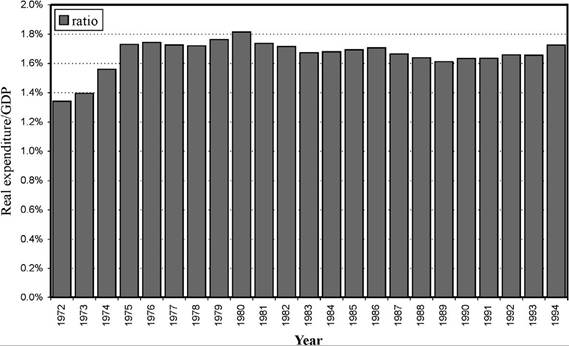
Figure 2. Pollution abatement costs, 1972-1994. PACE/GDP.
shown, pollution abatement costs as a fraction of GDP rise quite rapidly until 1980 and then remain relatively constant. As a fraction of overall output, these costs are relatively small. Generating a similar plot for costs as a fraction of manufacturing value-added produces similar results. Alternatively, if we consider pollution abatement costs specifically directed to the six criteria air pollutants and scale this by real U.S. output, the ratio is then incredibly small - approximately one half of one percent of GDP - and has remained so for over twenty years [see Vogan (1996)].18
Data from other countries supports the general conclusion that pollution abatement costs are a small fraction of GDP and show perhaps a slight upward trend. For example, total expenditures by both government and business in France rose from 1.2% of GDP in 1990 to 1.6% in 2000. Overthe 1991-1999 period, these same expenditures in Germany rose from 1.4% of GDP to 1.6%. Austria and The Netherlands show somewhat higher expenditures on the order of 2.1% and 1.6% in 1990 rising to 2.6% and 2.0% in 1998. While this data is clearly fragmentary, expenditures in the order of 1-2% of GDP seem to be the norm in OECD countries, with perhaps half of this being spent by private establishments and the remainderby governments.19
These figures however reflect to a certain degree the changing composition of output over time and therefore understate the impact higher pollution abatement costs have
is different in some respects from earlier ones. For details see the Survey of Pollution Abatement Costs and Expenditures, U.S. Census Bureau 1999 available at http://www.census.gov/econ/overview/mu1100/html.
18 These figures are also similar to those presented in the review of pollution abatement costs in Jaffe, Peterson and Portney (1995).
19 These data are drawn from the Organization for Economic Cooperation and Development 2003, “Pollution abatement and control expenditures in OECD countries”, OECD Secretariat, Paris. had on some industries. Levinson and Taylor (2003) for example argue that since the composition of U.S. manufacturing has been shifting towards less pollution intensive industries, aggregate measures understate the true costs of pollution regulations. They construct estimates of pollution abatement costs holding the composition of industry output fixed at the 2 and 3 digit industry levels and then compare these estimates with estimates allowing the composition of output to change. In all cases, holding the composition of U.S. output fixed in earlier periods leads to a higher estimate of industry wide abatement cost increases. As a result, the small increases in pollution abatement costs shown in the aggregate data are at least partially due to the U.S. shedding some of its dirtiest industries over time.
Our third and final fact is presented in Figures 3-8. These figures show a general tendency for emissions to at first rise and then fall over time. Since the U.S. exhibited trend growth in real per capita income of approximately 2% per year over this period, the time scale in the figures could just as well be replaced by income per capita. Note that the falling emissions/intensities reported in Figure 1 are necessary but not sufficient for this result. This pattern in the data is visible for all pollutants except nitrogen oxides that may at present be approaching a peak in emissions. Conversely, particulate pollution peaked much earlier than the other pollutants, while lead has a dramatic drop in the mid-1970s. These raw U.S. data support the contention that environmental quality at first deteriorates and then improves with increases in income per capita.
Another interesting aspect of these figures is the breakdown of emissions by enduse category. Apart from some exceptions arising from the miscellaneous category the within-pollutant source of the emissions remains roughly constant in many of the figures. For example, consider SO2. Aggregate emissions follow an EKC pattern, but the components of fuel combustion and industrial processes do as well. A similar pattern is found in volatile organic compounds, but less so in the case of carbon monoxide which
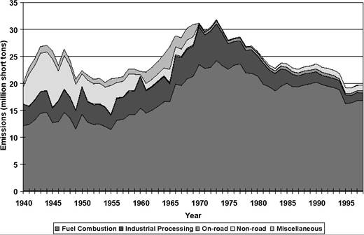
Figure 3. Sulfur dioxide emissions, 1940-1998.
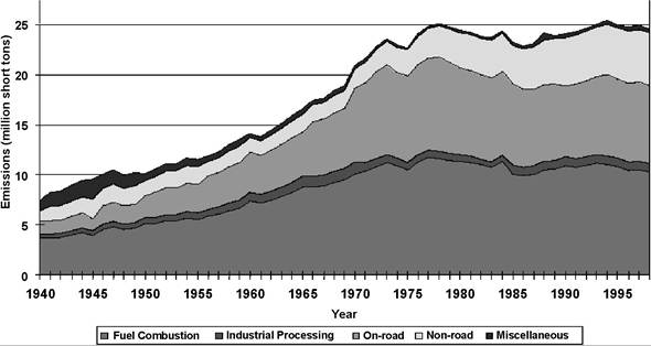
Figure 4. Nitrogen oxide emissions, 1940-1998.
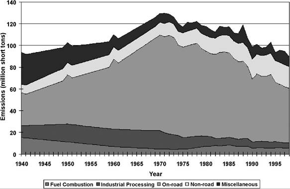
Figure 5. Carbon monoxide emissions, 1940-1998.
presumably is due to the change in automobile use over the period. In total the rough constancy in the within-pollutant sources of emissions suggests that the overall EKC pattern is not driven by strong compositional shifts.
Our finding of an EKC in the raw emission data is consistent with the recent flurry of formal empirical work linking per capita income and pollution levels. This empirical literature was fueled primarily by the work of Grossman and Krueger (1993, 1995) who found that, after controlling for other noneconomic determinants of pollution, measures
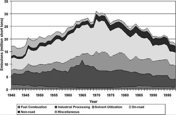
Figure 6. Volatileorganiccompounds, 1940-1998.
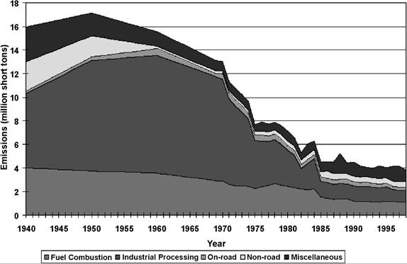
Figure 7. Particular matter PM10, 1940-1998.
of some (but not all) pollution concentrations at first rose and then fell with increases in per capita income.[487] Their work is important in several respects: it brought the empiri-
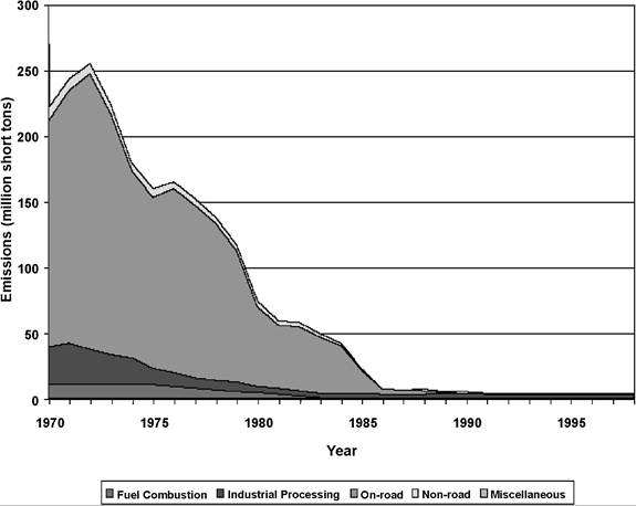
Figure 8. Leademissions, 1970-1998.
cal study of aggregate pollution levels into the realm of economic analysis; it debunked the commonly held view that environmental quality must necessarily decrease with economic growth; and it provided highly suggestive evidence of a strong policy response to pollution at higher income levels.
Unfortunately, empirical research has progressed very little from this promising start. Subsequent empirical research has focused on either confirming or denying existence of similar relationships across different pollutants.[488] Subsequent research has shown that the inverse-U relationship does not hold for all pollution, and there are indications the relation may not be stable for any one type of pollution.[489] Since the empirical work on the EKC typically employs cross-country variation in income and pollution to identify parameters, it is perhaps not surprising that there are signs of parameter instability. This instability could arise from country specific differences in the mechanism driving the two processes, but very little, if any, work has gone into evaluating the various hypotheses offered for the EKC. This interpretation of the econometric problems is of course consistent with our finding that the raw U.S. data offers a dramatic confirmation of Grossman and Krueger’s cross-country results. Cross-country differences leading to parameter instability are of course irrelevant in a one-country context.
In its original application, the EKC was interpreted as reflecting the relative strength of scale versus technique effects. However, it is difficult to support this interpretation. To isolate either the scale or technique effect we need to hold constant the composition of output, but this is not typically done in this literature. Therefore, the shape of the EKC may reflect some mixture of scale, composition and technique effects.
Despite these criticisms, the major and lasting contribution of this literature is to suggest a strong environmental policy response to income growth. The EKC studies are generally supportive of the hypothesis that income gains created by ongoing growth lead to policy changes that in turn drive pollution downwards. However, as our discussion in later sections will show, an EKC is compatible with many different underlying mechanisms and is entirely compatible with pollution policy remaining unchanged in the face of ongoing growth.
While most studies do not present evidence that allows us to distinguish between the underlying mechanisms responsible for the EKC, two recent studies offer additional insights. Hilton and Levinson (1998) examine the link between lead emissions and income per capita using a panel of 48 countries over the twenty-year period 1972-1992. This study is important because it finds strong evidence of an inverted-U-shaped relationship between lead emissions and per capita income, and then factors the changes in pollution into two different components. The first is a technique effect that produces an almost monotonic relationship between lead content per gallon of gasoline and income per capita. The second is a scale effect linking greater gasoline use to greater income.[490] This study is the first to provide direct evidence on two distinct processes (scale and technique effects) that together result in an EKC.
To interpret the empirical evidence as reflecting scale and technique effects one needs to rule out other possibilities. Although the authors do not couch their analysis in this context, their analysis implicitly presents the necessary evidence. First, they document a significant negative relationship between the lead content of gasoline and income per capita (post 1983). This relationship shows up quite strongly in just a simple crosscountry scatter plot of lead content against income per capita. Since lead content is arguably pollution per unit output, it is difficult to attribute the negative relationship to much other than income driven policy differences.[491]
Second, the authors find a hump-shaped EKC using data from the post-1983 period, but in earlier periods they find a monotonically rising relationship between lead emissions and income. The declining portion of the EKC only appears in the data once the negative health effects of lead had become well known. The emergence of the declining portion in the income pollution relationship is very suggestive of a strong policy response to the new information about lead. The fact this only appears late in the sample makes it difficult to attribute the decline in lead to other factors that could be shifting the demand for pollution. For example if the declining portion of the EKC was due to increasing returns to scale in abatement, then it should appear in both the pre- and post- 1983 data. If it was due to shifts in the composition of output arising naturally along the development path, why would it only appear in the post-1983 data? While it is possible to think of examples where these other factors are at play, the scope for mistaking a strong policy response for something else is drastically reduced in this study. The natural inference to draw is that the decline only occurs late in the sample because with greater information about lead’s health effects, policy tightened and emissions fell.
A second important study is Gale and Mendez (1998). They re-examine one year of sulfur dioxide data drawn from Grossman and Krueger’s (1993) study. The study does not offer a theory of pollution determination, but is original in investigating the role factor endowments may play in predicting cross-country differences in pollution levels. They regress pollution concentrations on factor endowment data from a cross-section of countries together with income-based measures designed to capture scale and technique effects. Their results suggest a strong link between capital abundance and pollution concentrations even after controlling for incomes per capita. Their purely cross-sectional analysis cannot, however, differentiate between location-specific attributes and scale effects. Nevertheless, their work is important because the strong link they find between factor endowments and pollution suggests a role for factor composition in determining pollution levels. That is, even after accounting for cross-country differences in income per capita, other national characteristics matter to pollution outcomes.
Combining our three stylized facts on pollution emissions presents us with an important question. How did aggregate emissions and emissions per unit output fall so dramatically in the U.S. without raising pollution abatement costs precipitously?
There are several possible explanations. One possibility is that ongoing changes in the composition of U.S. output have led to a cleaner mix of production that has lowered both aggregate measures of costs and emissions. The downward trend in emissions per unit output shown in Figure 1 prior to the advent of the Clean Air Act suggests some role for composition effects. While changes in the composition of U.S. output are surely part of the story, there are reasons to believe that they cannot be the most important part. Over the 1971-2001 period of active regulation by the EPA, total emissions of the 6 criteria air pollutants (nitrogen dioxide, ozone, sulfur dioxide, particulate matter, carbon monoxide and lead) decreased on average by 25%. Over this same period, gross domestic product rose 161% and pollution abatement costs have risen only slightly.[492] The magnitude of these emission reductions is too large for it to reflect composition changes alone.
To get a feel for the magnitudes involved note that if changes in the composition of output over the 1971-2001 period are to carry all the burden of adjustment, then we would set the changes in ai to zero in (2). Then using the EPA’s estimate of an average 25% reduction for E and the 161% increase for Y, we find that the weighted average of industry level changes must add up to - 186% change. This is just too large a realignment in the composition of industry to be credible.
It is also apparent from the figures that emissions for most pollutants have been falling since the early 1970s and as we saw earlier there are limits to how far aggregate emissions can fall via composition effects. Our earlier discussion of the static nature of the within-pollutant sources of emissions also argues against strong composition effects. Finally, there is little evidence that international trade is playing a major role in shifting dirty goods industries to other countries but stronger composition effects after the advent of federal policy in early 1970s would be necessary to explain the fall in emissions seen in the figures.[493] For this set of reasons it seems clear that composition effects alone cannot be responsible for the result.
Another possible explanation is that ongoing growth in incomes has generated a strong demand for environmental improvement. In this account, income gains over the post-World War II period produce a change in policy in the early 1970s and usher in the EPA and the start of emission reductions. While this explanation fits with the decline in emission to output ratios and the lowered emissions since the early 1970s, it too cannot be the entire story. As we discuss in Section 4, if rising incomes are to be wholly responsible for the change in pollution policy, agents must being willing to make larger and larger sacrifices in consumption for improving environmental quality. For example, the theory models of Stokey (1998), Aghion and Howitt (1998), Lopez (1994), etc. all require a rapidly declining marginal utility of consumption to generate rising environmental quality and ongoing growth. But as Aghion and Howitt note:
Thus it appears that unlimited growth can indeed be sustained, but it is not guaranteed by the usual sorts of assumptions that are made in endogenous growth theory. The assumption that the elasticity of marginal utility of consumption be greater than unity seems particularly strong, in as much as it is known to imply odd behavior in the context of various macroeconomics models... (p. 162).
A rapidly declining marginal utility of consumption is required in earlier work because increasingly large investments in abatement are required to hold pollution in check[494] This implies the share of pollution abatement costs in the value of output approaches one in the limit, which is inconsistent with available evidence.[495]
A final possibility is technological advance. Ongoing technological progress in production and abatement could simultaneous drive long run growth and hold pollution abatement costs in check. Technological progress in goods production could be the driving force for growth in final output, while technological progress in abatement allows emissions per unit of output to fall precipitously without raising environmental control costs skyward. In this explanation, income gains from ongoing growth are responsible for the onset of serious regulation in the 1970s, but the advent of regulation then brought forth improvements in abatement methods. As a consequence agents have not been required to make increasingly large sacrifices in consumption for improving environmental quality. As we show in Section 4, this explanation is consistent with the predictions of both our Green Solow and Kindergarten models.
Before we proceed we should note that the stylized facts given thus far exclude a discussion of many other pollutants. By selecting only pollutants for which data is available we may have erred on the side of optimism since the measurement of pollutants is almost always a precursor to their active regulation. One important omission from the above is any discussion of air toxics such as benzene (in gasoline), perchloroethylene (used by dry cleaners), and methyl chloride (a common solvent). These are chemicals are believed to cause severe health effects such as cancer, damage to the immune system, etc. At present the EPA does not maintain an extensive national monitoring system for air toxics, and only limited information is available.[496]
Another omission is any discussion of the set of long-lived chemicals and chemical by-products that have found their way into waterways, soils and the air. These products have very long half-lives and produce serious health and environmental effects. Prominent among these in U.S. history are DDT, PCBs, lead, and most recently CFCs. Official estimates on emissions of these pollutants is difficult to find, but historical accounts and partial data indicate their emissions follow a pattern roughly similar to that of lead shown in Figure 8. As shown by the figure the history of lead is one of strong initial growth in emissions, followed by a rapid phase-out and virtual elimination. In fact, lead continues to be emitted in small amounts, whereas PCB emissions rose from very low production levels in the 1930s to millions of pounds per year of production in the 1970s, to end with a complete ban in 1979. Similarly, DDT was used extensively after World War II but banned in 1972. CFC production in the U.S. rose quickly with the advent of refrigeration and air conditioning, but this set of chemicals now faces a detailed phaseout with CFC-11 and CFC-12 already facing a complete production ban. The salient feature of these accounts is strong early growth followed by quite rapid elimination.
A final failing of these data is that they are on emissions and not concentrations.[497] Concentration data is available for most of these data at least over the last 20-30 years, but the data is well known to be noisy and suffers from other problems related to comparability over time. Nevertheless most aggregate measures of air quality in cities have been improving over time. For example, data on the number of U.S. residents living in counties that were designated nonattainment because of their failure to achieve federal air quality standards shows that over the 1986 to 1998 period these numbers have been falling quite dramatically for sulfur dioxide, nitrogen oxide, carbon monoxide, lead and PM10. The number of people living in counties who failed the federally mandated ozone air quality has however risen from 75 million in 1986 to 131 million in 1998.[498]
2.
More on the topic Preliminaries:
- Preliminaries
- C Preliminaries to marriage: age, betrothal, and consent
- Preliminaries
- EPILOGUE Muddling Through: Freedom of Expression in the Absence of a Human Right
- The Law of Marriage - BriefHistory
- 4 Contracting out
- In the fourth and fifth centuries, Roman marriage law takes on quite a different appearance from the “classical” law of the first three centuries.
- Staging a Massacre
- Ukraine in the Age of Globalization
- Contents