The baby bust and baby boom
Two facts stand out about the fertility of American women. First, it has dropped drastically over the last two hundred years. This decline is called the demographic transition, but will be labeled here the baby bust.
Second, the secular decline in fertility has had only one interruption, the baby boom. These two facts can easily be accounted for within the context of the neoclassical growth model. Just two modifications to the standard model are required: a fertility decision needs to be added, and household production incorporated.2.1. Theenvironment
Imagine a small open economy populated by overlapping generations.5 People live for three periods, one period as children and two as adults. Young adults are endowed with one unit of time. They can use this time for either working or raising kids. An individual is fecund only in the first period of adulthood. Old agents are retired.
Tastes. The lifetime utility function for a young adult is given by

where cy and co' denote the adult’s consumption when young and old, and ny represents the number of kids that he would like to have when young. The constant c proxies for the household production of market goods. As will be seen, it plays an important role in the analysis.
Income. Young agents work for the market wage w. They save for old age at the internationally determined time-invariant gross interest rate r.
Cost of children. Children are expensive. The production function for children is given by
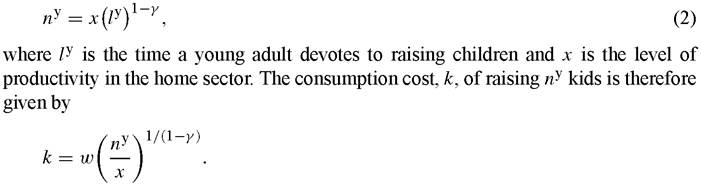
The cost of raising children is directly proportional to the wage rate.
5 The model presented here is based on Greenwood, Seshadri and Vandenbroucke (2005).
The young agent's choice problem.
The decision problem facing a young adult is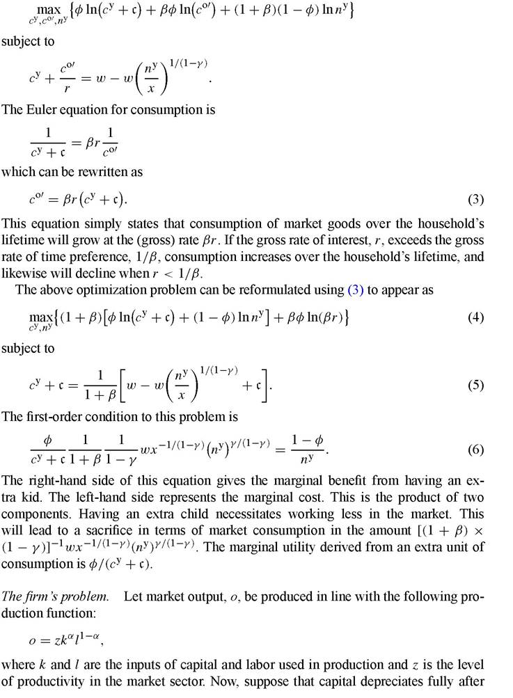
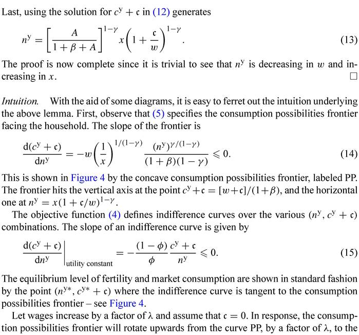
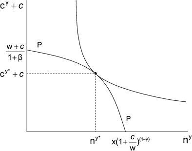
Figure 4. The determination of fertility.
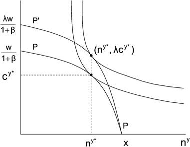
Figure 5. The effect of an increase in wages on fertility when c = 0.
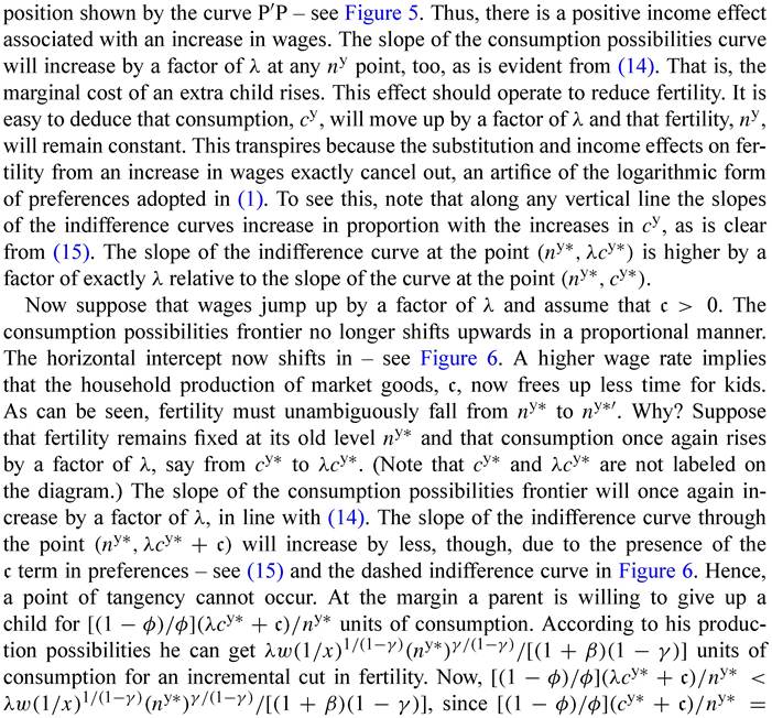
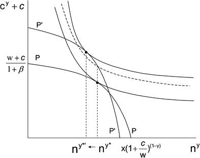
Figure 6. The effect of wages on fertility when c = 0.
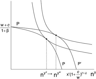
Figure 7. The effect of an improvement in household technology on fertility.
Corollary. Fertility, ny, is decreasing in the level of market productivity z. (Fertility is increasing in the international rate of return r.)
Example 1 (Fertility, 1800 and 1940). Assignthe following parameter values to the model.
(i) Tastes: β = 0.9420, φ = 0.47, c = 2.97.
(ii)Technology: α = 0.33, γ = 0.33, r = 1/â.
Normalize the level of market and home productivity for the year 1800 to be unity. That is, set x = z = 1.0 for 1800. With this configuration of parameter values, Equation (16) predicts that the level of fertility per adult should be 3.5, exactly the value observed in the U.S. in 1800 - at that time a married couple experienced 7 births on average.
Now, between 1800 and 1940 market productivity grew by a factor of 3.5. So, reset z to equal 3.5 for 1940. The model predicts that fertility should fall to 1.2. It actually fell to 1.1.[1] The intuition is obvious since w, the wage rate, is increasing in z and decreasing in r.
The baby boom. Once again presume that market productivity is growing over time at the constant rate z'/z = ζ > 1. Now imagine that a once-and-for-all jump in household productivity happens. According to (13), fertility will jump up on this account. After this innovation fertility will revert back to its old time path of monotonic decline.
Example 2 (Fertility, 1960 and 2000). Keep the parameter values from the previous example. U.S. fertility per prime-age adult (males plus females) rose from 1.1 to 1.8 between 1940 and 1960. This was the baby boom. By 1960 market-sector TFP had risen to 4.9, so now reset z = 4.9 for 1960. Using (16) it is easy to deduce that a fertility rate of 1.8 can be obtained by letting x = 1.8. That is, the baby boom can be generated by assuming that household-sector productivity grew by a factor 1.8 between 1940 and 1960. Finally, U.S. TFP had risen to 7.4 by the year 2000. The model predicts that the fertility rate should be 1.5, as opposed to the observed rate of 1.0.
3.