The U.S. demographic transition

At the start of the nineteenth century most adult males worked in the agricultural sector and children got very little in the way of a formal education. By the end of the twentieth century almost no adult worked in agriculture, at least relative to nonagriculture.

3.1. Theenvironment

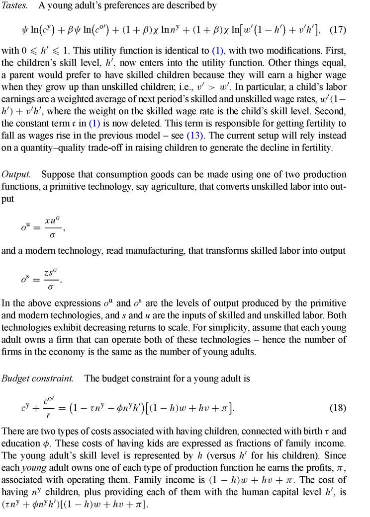
Take the setup of the previous section with two slight modifications.^[146] First, assume that parents now care about the quality of their children in addition to the quantity of them. Second, suppose that there are two production sectors in the economy. One sector uses solely skilled labor, the other only unskilled workers. A unit of skilled labor earns the wage v, while a unit of unskilled labor gets w. A parent must choose the skill level to endow his offspring with (or the quality of his children).

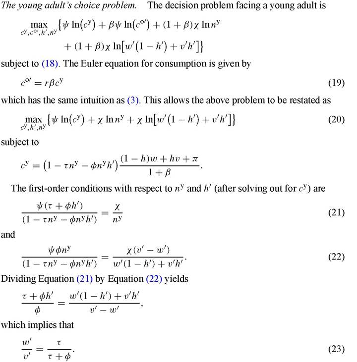
In other words, tomorrow’s skill premium is a constant, pinned down by the proportional costs for birth and education. Note that this follows directly from the assumption that quantity and quality have same weight χ in the utility function.

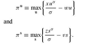
The firms' problems. The firms in the agricultural and manufacturing sectors will solve the problems

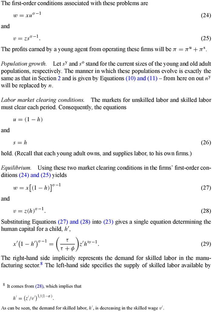
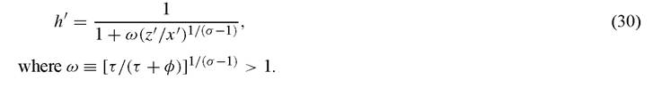
freeing up workers from agriculture.⁹ This equation can be solved to get a closed-form expression for the level of human capital that reads

3.2. Analysis

Now, imagine that the economy is resting in a steady state where z' and χ' are constant. It is then easy to see from (30) that h' will be constant. Notice that if Z and χ' were to increase at the same rate, h' would also remain unchanged. This result follows be­cause identical increases in total factor productivity in both sectors leave unchanged the demand for each type of labor, given the constancy of the skill premium. This leaves un­changed the fraction of total labor allocated to each sector. So, when will human capital rise?

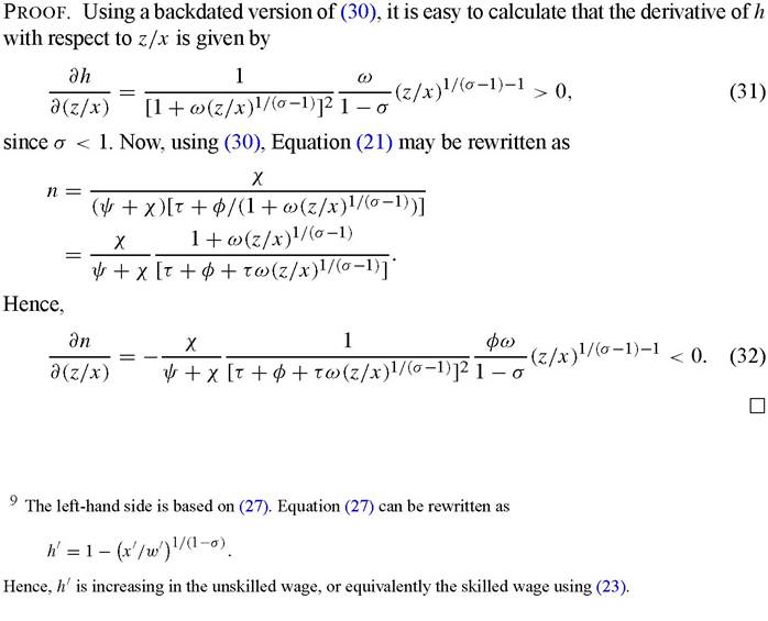
Lemma 2. As TFP in manufacturing, z, rises relative to agriculture x, human capi­tal, h, increases and fertility, n, falls.

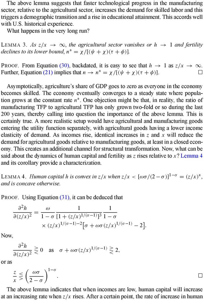
capital will slow down, and human capital will increase at a decreasing rate as z/x rises. Thus, the convergence of h from a society where every individual is unskilled (h = 0) to one in which every one is skilled (h = 1) will have an S shape that is characteristic of the diffusion of many innovations. Now, recall that fertility is inversely related to human capital. Consequently, fertility will initially fall at a increasing rate, and then will eventually decline at an decreasing rate as it converges to n*. The following corollary characterizes the dynamics of fertility.

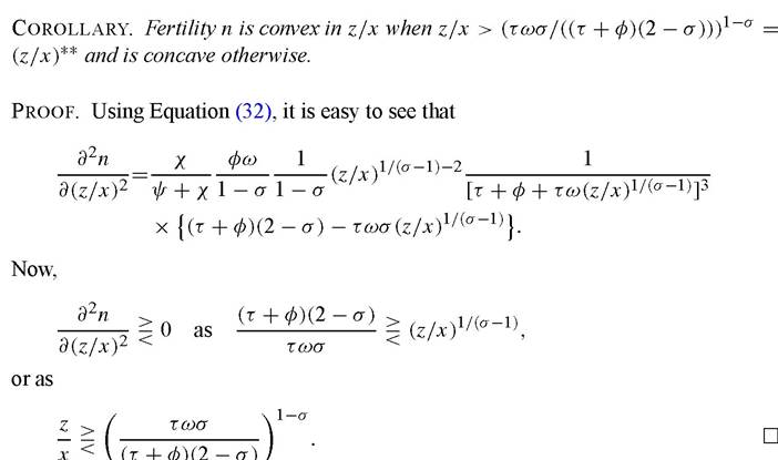
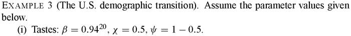
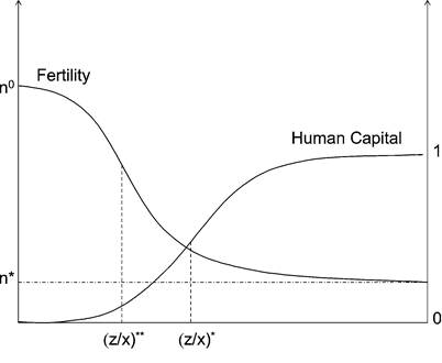
Figure 8. The dynamics of fertility and human capital.

(ii)Technology: σ = 0.8.

(iii) Child care: τ = 0.123, φ = 0.4.

The time is 1800. Assume that (z∕x) ₁₈oo = 2.36. Then, Equation (30) implies that h₁₈₀₀ = 0.05; i.e., about 5 percent of the population are skilled. The rest of the population, 95 percent, live in the rural sector. Further, Equation (21) implies that n₁₈₀₀ = χ∕[(ψ + χ)(τ + φh ₁₈₀₀)] = 3.5, which is exactly the number of kids per adult (male plus female) in 1800. An average married couple in 1800 had 7 kids. Now, move ahead to 1940. TFP in agriculture grew by a factor of 1.95, while TFP in manufacturing grew by a factor of 4.11. Consequently, (z∕x)₁₉₄₀ = (4.11/1.95) ? (z∕x)₁₈₀₀ = 4.97. Now, Equation (30) implies that h₁₉₄₀ = 0.69, or that about 31 percent of the popu­lation live in the rural sector. Further, n₁₉₄₀ = χ∕[(ψ + χ)(τ + φh₁₉₄₀)] = 1.26, so that an average family has 2.52 children (as opposed to 2.23 in the data). Finally, the long-run value of fertility is n* = 0.96. In the long run an average family will give birth to 1.92 children.

Notice that even without employing any differences in curvature between manufac­turing or agricultural goods, or differences in the skill intensities associated with the production of these goods, technological advance can account for most of the decline in fertility between 1800 and 1940.^[147]

4.