The integrated economy

Imagine a world without borders, a world in which all goods and factors can be trans­ported across different regions at negligible cost. Some industries spread their produc­tion process across many regions searching for the ideal environment for each specific phase of production.

The integrated economy provides a natural benchmark for the study of economic growth in an interdependent world. Moreover, its simplicity and elegance encapsulates the essence of what growth theory is all about: deriving strong results using minimal­ist models. In the spirit of the so-called “new growth theory”, I shall use a model that jointly determines the stock of capital and the level of technology. Admittedly, the model is somewhat lopsided. On the one hand, it contains a fairly sophisticated formulation of technology that includes various popular models as special cases. On the other hand, it uses a brutal simplification of the standard overlapping-generations model as a descrip­tion of preferences. Despite this, I do not apologize for the imbalance. A robust theme in growth theory is that the interesting part of the story is nearly always on the technology side, and rarely on the side of preferences.

This section develops the basic framework that I use throughout the chapter. Sec­tion 1.1 describes the integrated economy, while Section 1.2 derives its main predictions for world growth. Section 1.3 goes back to a period in which all the regions of the world lived in autarky, and compares the growth process of this world with the integrated economy. This is just the first of various attacks to the question of globalization and its effects on the world economy.

1.1. A workhorse model

Consider a world economy inhabited by two overlapping generations: young and old. The young work and, if productive, they earn a wage. The old retire and live off their savings. All generations have size one. There are many final goods used for consumption and investment, indexed by i ∈ I. When this does not lead to confusion, I shall use I to refer both to the set of final goods and also to the number of final goods. As we shall see later, the production of these final goods requires a continuum of intermediate inputs. There are two factors of production: labor and capital. For simplicity, I assume capital depreciates fully within one generation.^[280] The world economy contains many regions. But geography has no economic consequences since goods and factors can be transported from one region to another at any time at negligible cost.

The citizens of this world differ in their preferences and access to education. S_t mem­bers of the generation born in date t are patient and maximize the expected utility of old age consumption, while the rest are impatient and maximize the expected utility of con­sumption when young. The utility function has consumption as its single argument, and it is homothetic, strictly concave and identical for all individuals. H_t members of the generation born in date t can access education and become productive, while the rest have no access to education and remain unproductive.^[281] I refer to S_t and H_t as “sav­ings” and “human capital”, and I allow them to vary stochastically over time within the unit interval.

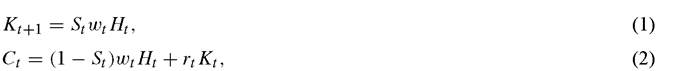
where K_t and C_t are the average or aggregate capital stock and consumption, and w_t and r_t are the wage and rental rate of capital. Equation (1) states that the capital stock equals the savings of the young, which consist of the wage of those that are patient and productive. The assumption that capital depreciates fully in one generation implies that the capital stock is equal to investment. Equation (2) says that consumption equals the wage of the impatient and productive young plus the return to the savings of the old.^[282]

Consumption and investment can be thought of as composites or aggregates of the different final goods. A very convenient assumption is that both composites take the same Cobb-Douglas form with spending shares that vary across industries, i.e. σ_i with ∑_i∈₁ σ_i — 1. Since there is a common ideal price index for consumption and invest­ment, it makes sense to use it as the numeraire and this implies that aggregate spending

where E_it and P_it are the total spending on and the price of the final good of indus­try i. Equation (3) states that spending shares are constant, while Equation (4) sets the common price of consumption and investment equal to one.

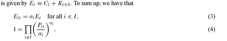
Production of final goods uses labor, capital and a continuum of different varieties of intermediate inputs, indexed by m ∈ [0, M_it ] for all i ∈ I.As usual, I interpret the measure of input varieties, M_it for all i ∈ I, as the degree of specialization or the technology of the industry. This measure will be determined endogenously as part of the equilibrium.

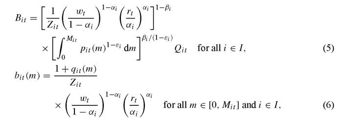
where 0 ≤ β_i ≤ 1, ε_i > 1 and 0 ≤ a_i ≤ 1, Q_it is total production of final good i, q_it(m) and p_it(m) are the quantity and price of the mth input variety of industry i, and the variables Z_it are meant to capture the influence on industry productivity of geography, institutions and other factors that are exogenous to the analysis.^[283] I loosely refer to the Z_it ^,s as “industry productivities” and assume they vary stochastically over time within a support that is strictly positive and bounded above. Equation (5) states that the technology to produce the final good of industry i is a Cobb-Douglas function on human and physical capital, and intermediate inputs. The latter are aggregated with a standard CES function. Equation (6) states that the production of intermediates is also a Cobb-Douglas function on human and physical capital, and that there are fixed and variable costs.^[284] I interpret the fixed costs as including both the costs of building a specialized production plant and the costs of inventing or developing a new variety

¹⁰ This assumption is crucial for tractability, since it eliminates a potentially large set of state variables, i.e. Mit for all i ∈ I.

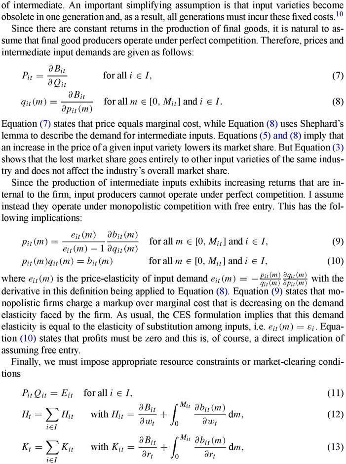
where H_it and K_it are the labor and capital demanded by industry i. Since the integrated economy is a closed economy, Equation (11) forces the aggregate supply of each good to match its demand, while Equations (12)-(13) state that the aggregate supply of labor and capital must equal their demands. The latter are the sum of their industry demands, and these are calculated using Shephard’s lemma.

This completes the description of the model. For any admissible initial capital stock and sequences for S_t, H_t and Z_it, an equilibrium of the integrated economy consists of sequences of prices and quantities such that Equations (1)-(13) hold in all dates and states of nature. The assumptions made ensure that this equilibrium always exists and is unique. I shall show this by construction in the next section.

The reader might be wondering why I have not formally introduced financial markets. I have allowed individuals to construct their own capital and use it as a vehicle to carry on their savings into retirement (a world of family-owned firms?). But I have not allowed them to trade securities in organized financial markets. The reason is simply to save notation. The assumptions made ensure that asset trade does not matter in this world economy.¹¹ To see this, assume there exist sophisticated financial markets where all individuals can trade a wide array of state-contingent securities. Naturally, the old would not be able to trade these securities since they will not be back to settle claims one period later. But the young would not trade with each other either. Impatient young would not be willing to trade securities since they do not have income in their old age and are happy to consume all their income during their youth. Patient young are the only ones willing and able to trade these securities. But they all have identical preferences and face the same distribution of returns to capital, and therefore they find no motive to trade with each other. Thus, we can safely assume the integrated economy contains sophisticated financial markets that allow individuals to enter contracts that specify exchanges of various quantities of the different goods to be delivered at various dates and/or states of nature. It just happens that these financial markets do not make any difference for consumption and welfare.

1.2. Diminishing returns, market size and economic growth

To study the forces that determine economic growth in the integrated economy, it is useful to start with a familiar expression

^[1] This statement is not entirely correct.

istic” world. There is a unique steady state and the stock of physical capital converges monotonically towards it from any initial position. The steady state is stable because in­creases (decreases) in the stock of physical capital lower (raise) the output-capital ratio and lead to a lower (higher) growth rate. The bottom panel shows that the “stochastic” world exhibits similar dynamics, with the stock of physical capital monotonically con­verging to a steady state interval, rather than a steady state value. Once the stock of physical capital is trapped within this interval, its growth rate fluctuates between pos­itive and negative values and averages zero in the long run. These examples illustrate why sustained growth is not possible if diminishing returns are strong and market size effects are weak.

¹⁵ Note that μ(1 — α) — υ ^p 0.

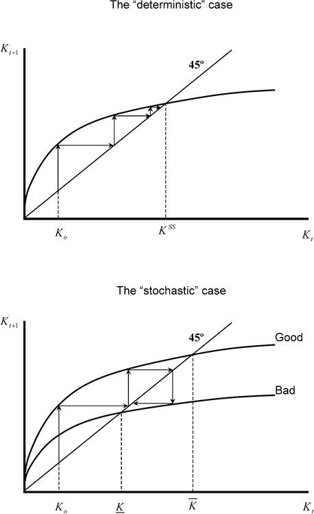
Figure 5. αμ + υ < 1. Notes. This figure shows the case of strong diminishing returns and weak market size effects. In the top panel, the stock of physical capital converges monotonically to its unique steady state. The bottom panel shows the stochastic case, where the stock of physical capital converges to the steady state interval [ K, K ] within which it fluctuates according to the states of the world.

Figure 6 shows the case in which diminishing returns are weak and market-size ef­fects are strong, i.e. μα + υ ≥ 1. The top panel shows the “deterministic” world again. There is unique steady state that is unstable. If the stock of physical capital starts above the steady state, it grows without bound at an accelerating rate. If it starts below, the stock of physical capital contracts over time also at an accelerating rate. The steady state is now unstable because increases (decreases) in the stock of physical capital raise

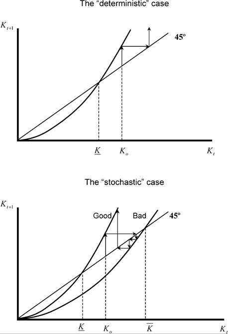
Figure 6. αμ + υ > 1. Notes. This figure shows the case of weak diminishing returns and strong market size effects. In the top panel, the stock of physical capital grows at increasing rates since K_o > K. In the bottom panel the stock of physical capital fluctuates between K and K according to the states of the world, until it eventually leaves this range.

(lower) the output-capital ratio and lead to a higher (lower) growth rate. The bottom panel shows that the “stochastic” world also exhibits similar dynamics. One difference however is that there is no steady state. Instead, there is a threshold interval. If the stock of physical capital is above (below) this interval, it grows (contracts) at an accelerat­ing rate. If the stock of physical capital starts within the threshold interval, it fluctuates within it until it eventually exits. This happens with probability one, and only luck de­termines when this exit occurs and whether the world economy exits above and enters an expansionary path or, alternatively, it exits below and enters a contractionary path. Therefore, sustained growth is possible (but not necessary) if diminishing returns are weak and market size effects are strong.

This model suggests a simple account of the history of the world economy since the 1500s. It is based on the “stochastic” world of Figure 6 and it goes as follows: for centuries, the size of the world economy was too small to generate sustained growth. Located within the threshold interval, the world economy was subject to periodic ex­pansions and contractions with virtually zero average growth. This is consistent with Maddison’s calculation that the world economy grew only about eighteen percent from 1500 to 1820. But this was an unstable situation in the very long run. The Industrial Revolution marks the moment in which, after a series of favorable shocks, the world economy reached enough size to exit the threshold interval and started traveling on the path of accelerating growth reported in Figure 1. As a result of this successful exit, the world economy grew more than seven hundred and fifty percent from 1820 to 1998.

Although suggestive, this account is far too sketchy and incomplete to be taken seri­ously. Moreover, I find highly improbable that the last five hundred years of the world economy can be understood in terms of a model that postulates negligible costs of transporting goods and factors and constant world population. Surely the demographic revolution and the process of globalization have both played central roles in shaping the growth process during this period. This chapter is not the place for a discussion of the growth effects of the demographic revolution.¹⁶ But it is definitely the place to study the growth effects of globalization, and we turn to this topic next.

1.3. The effects of economic integration

Assume the world economy initially consisted of many regions or locations separated by geographical obstacles that made the costs of transporting goods and factors among

^[1] Equation (26) follows from adding the income from human and physical capital of the inhabitants of the region, and noting that aggregate or world shares of human and physical capital are constant and equal to 1 — α and α, respectively. Equation (27) follows from Equations (1) and (23), and the observation that wages are the same for all productive workers of the world. Without loss of generality, I keep assuming that there is no trade in securities.

^[1] To derive this expression I have assumed a zero cross-industry correlation between αi and μ/, i.e. υ = 0. This parameter restriction is useful because it allows us to unambiguously disentangle the “increased-market- size” and “improved-factor-allocation” effects.

These gains can be decomposed into three sources corresponding to each of the terms of Equation (28). The first one shows the growth of income that results from moving industries from low to high productivity locations. This term would vanish if region c had the highest productivity in all industries. The second term shows the growth of in­come that results from relocating factors away from those regions and/or industries in which they were abundant in autarky into those in which they were scarce. This term would vanish if region c had world average factor proportions. The third term shows the growth in income that is due to an increase in market size that allows industries to support a higher degree of specialization. This term would vanish if the size of re­gion c were arbitrarily large with respect to the rest of the world. An implication of Equation (28) is that the static gains from economic integration are greater for regions with low productivity, extreme factor proportions and modest amounts of physical and human capital.

If coupled with an appropriate transfer scheme, globalization leads to a Pareto im­provement in the world economy. Equation (28) shows that, with the same production factors, the integrated economy generates more output than the world of autarky. It is therefore possible to implement a transfer scheme that keeps constant the income of all current and future young and gives more income to all current and future old. Under this transfer scheme, investment and the stock of physical capital would be unaffected by economic integration. But the production and consumption of all generations born at date t = 0 or later would increase. Of course, there exist many alternative transfer schemes that ensure that globalization benefits all. Moreover, since each region gains from trade there exist Pareto-improving transfer schemes that can be implemented with­out the need for inter-regional transfers. That is, ensuring that globalization generates a Pareto improvement does not require compensation from one region to another.

How “large” the transfer scheme must be to ensure that economic integration leads to a Pareto improvement? The answer is “not much” if most of the gains from economic integration come from higher productivity and increased market size. The reason is that in this case all factors share in the gains from integration. The required transfer scheme could be “substantial” if the gains from integration come mostly from improved factor allocation. This is because within each region the owners of the abundant factor obtain more than proportional gains from integration while the owners of the region’s scarce factor might have losses. In this case, implementing a Pareto improvement requires a transfer from the former to the latter.

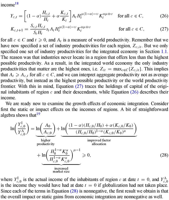
Without a transfer scheme, it is relatively straightforward to trace the dynamic effects of economic integration. Assume for simplicity that the world contains many symmetric regions so that before integration all of them had the same law of motion. The top panel of Figure 7 shows the effects of economic integration in the “deterministic” world when diminishing returns are strong and market size effects are weak. Economic integration raises the steady state stock of physical capital and sets up a period of high growth that eventually ends. It is straightforward to see that the effects would be similar in the “sto­chastic” world, with economic integration permanently raising the steady state interval. Using the jargon of growth theory, if μα + υ < 1 economic integration has level effects

Figure 7. Effects of economic integration. Notes. This figure illustrates the effects of economic integration. The top panel shows that, if aμ + υ < 1, economic integration has level effects on income. The bottom panel shows that, if aμ + υ > 1, economic integration has growth effects on incomes.

on income. The bottom panel of Figure 7 shows the opposite case in which diminishing returns are weak and market size effects are strong. In this case, economic integration shifts down the steady state value, increasing the growth rate permanently. Once again, it is straightforward to see that the effects would be similar in the “stochastic” world, with trade shifting the threshold interval to the left. Using again the jargon of growth theory, if μa + è ≥ 1 integration has growth effects on income.

It is tempting now to revisit our earlier account of the history of the world economy since the 1500s, and propose an alternative version which is also based on the “sto­chastic” world with μa + υ > 1. It goes as follows: for centuries, the world economy consisted of a collection of autarkic regions that were too small to sustain economic growth. Located within the threshold interval, these regions were subject to periodic expansions and contractions with virtually zero average growth. Once again, this is consistent with Maddison's calculation that the world economy grew only about eigh­teen percent from 1500 to 1820. The Industrial Revolution occurs when a series of reductions in trade costs between some British regions raised their combined size above the threshold interval and set them on the path of accelerating growth. As time went on, more and more regions joined the initial core and the Industrial Revolution spread throughout Britain and moved into France, Germany and beyond. It is therefore a reduc­tion of trade costs and the progressive extension of markets that made possible sustained growth and allowed the world economy to grow more than seven hundred and fifty per­cent from 1820 to 1998. This might also explain why this growth in world income was accompanied by an even higher growth in world trade.^[285]

This view of the development process is also broadly consistent with the general ob­servations about inequality between center and periphery discussed in the introduction. Regions that join the integrated economy (the “center”) become rich and take off into steady growth. Regions that do not join the integrated economy (the “periphery”) are left behind, technologically backward and capital poor. As more and more regions enter the integrated economy, those that are left behind become relatively poorer and world inequality increases. Eventually all regions will enter the integrated economy and world inequality will decline. Therefore, this model generates an inverted-U shape or Kuznets curve, with world inequality rising in the first stages of world development and declining later. Pritchett (1997), Bourguignon and Morrisson (2002) and others have shown that world inequality has increased from 1820 to now. It remains to be seen if this inequality will decline in the future.

This stylized model also illustrates some of the conflicts that globalization might cre­ate. It follows from Equation (28) that the gains from trade are large for regions whose factor proportions are far from the world average. Ceteris paribus, this means that re­gions in the center would like that new entrants into the integrated economy to move the world average factor proportions away from them. In fact, unless productivity and mar­ket size effects are substantial, the entry of a large region creates losses to other regions with similar factor proportions. This implies, for instance, that the Chinese process of economic integration should be seen with some concern in countries with similar factor proportions such as Mexico and Indonesia, but with hope in the European Union or the United States.

This view of globalization and growth leads to a powerful prescription for economic development: open up and integrate into the world economy. I believe this is a funda­mentally sound policy prescription, and history is largely consistent with it. But there are a number of important qualifications that this stylized model cannot capture. Integrating into the world economy is not an “all-or-nothing” type of affair in which regions move overnight from autarky to complete integration. The process of economic integration is slow and full of treacherous steps. Obtaining general prescriptions for development in a world of imperfect integration has proved to be a much more challenging task. I shall come back to this important point later, but we must first introduce trade frictions into the story.

2.