Specialization, trade and diminishing returns

Let us revise our model of globalization. As in Section 1.3, assume that at date t = 0 the costs of transporting goods across regions suddenly fall from prohibitive to negligible.

Assuming that human capital is immobile internationally is somewhat dubious, as there are some well-known examples of large contingents of people working overseas. But most of the results discussed here would go through with only minor changes under the weaker and reasonably realistic assumption that international flows of people are quantity constrained, although not necessarily at zero.^[286] Assuming that physical capital is immobile is appropriate for buildings and structures and, probably, not too unreason­able for the most important types of machinery and equipment. Moreover, assuming that existing physical capital cannot be transported does not preclude physical capital to effectively “move” across regions over time, as it declines in some regions through depreciation and increases in others through investment.^[287]

If physical capital is immobile, pieces of capital located in different regions might offer different return distributions. This opens up a role for financial markets. Although the old and the impatient young still have no incentive to trade securities, the patient young now have a motive. Those that are located in regions where physical capital offers an attractive distribution of returns want to sell securities and use the proceeds to finance additional purchases of domestic physical capital.

Despite this, I will not let international financial markets play this role. This failure of financial markets could be due to technological motives or informational problems of various sorts. But I prefer instead to think of it as being caused by lack of incentives to enforce international contracts. In the integrated economy, individuals could enter into contracts that specify exchanges of various quantities of the different goods to be delivered at various dates and/or states of nature. It is standard convention to refer to the signing of contracts that involve only contemporaneous deliveries as “goods” trade, while the signing of contracts that involve future (and perhaps state contingent) deliv­eries is usually referred to as “asset” trade. Both types of trade require sufficiently low costs of transporting goods. But asset trade also requires that the signing parties cred­ibly commit to fulfill their future contractual obligations. The domestic court system punishes those that violate contracts, thus creating the credibility or trust that serves as the foundation for domestic financial markets. But there is no international court system that endows sovereigns with the same sort of credibility, and this hampers international financial markets. I assume next this problem is so severe that it precludes all asset trade.

Unlike the integrated economy, in the world analyzed in this section each region’s total production, spending and capital stock are always determined. Since trade balances and current accounts are zero, the income of each region equals the value of both its production and spending, i.e.

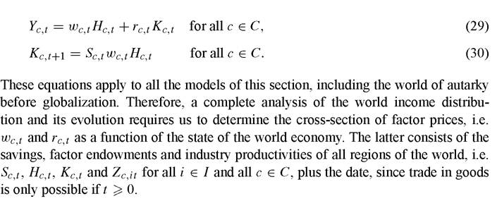
The rest of this section is organized as follows. Section 2.1 studies further the world of autarky, while the rest of the section studies the world after globalization. In Section 2.2, we explore a world in which frictions to factor mobility and asset trade are not binding after globalization. Section 2.3 provides a formal description of the model. Sections 2.4 and 2.5 examine worlds where frictions to factor mobility and asset trade remain binding after globalization.

productivity. Positive (and permanent) shocks to any of these variables raise the region’s capital stock and income. As Equation (34) shows, these shocks have growth effects if αμ + υ '≥ 1, but only have level effects if αμ + υ < 1. Regardless of the case, the effects of these shocks never spill over to other regions.

Assume the joint distribution of savings, human capital and industry productivities is stationary. Then, Equations (33) and (34) imply a strong connection between the cross­sectional and time-series properties of the growth process. If diminishing returns are strong and market size effects are weak, i.e. if μα + υ < 1, world average income (Y_t) and its regional distribution (Y_c,t∕Yt) are both stationary. If instead diminishing returns are weak and market size effects are strong, i.e. μα + υ > 1, world average income and its regional distribution are both nonstationary. This result provides a tight link between the long run properties of the growth process and the stability of the world income distribution.

It is commonplace among growth theorists to interpret cross-country data from the vantage point of the autarky model.^[288] One influential example is the work of Mankiw, Romer and Weil (1992). They combined Equations (33) and (34) to obtain an equation relating income to savings, human capital, country productivity, and lagged income; and estimated it using data for a large cross-section of countries. They interpreted the residuals of this regression as measuring differences in country productivities and mea­surement error, and concluded that differences in savings and human capital explain (in a statistical sense) about 80 percent of the cross-country variation in income. Their pro­cedure imposed the restriction μ = 1 (and therefore υ = 0) and yielded an estimate of α of about two thirds. Hall and Jones (1999) and Klenow and Rodriguez-Clare (1997) in­terpreted this high estimate of α as a signal that the regression was miss-specified. Their argument was that savings, human capital and productivity were positively correlated and the omission of productivity from the regression biased upwards the estimate of α. These authors used Equations (33) and (34) to calibrate country productivities keeping the assumption that μ = 1, but instead imposing a value of α of about one third.^[289] With these productivities at hand, they found that about two thirds of the variation in incomes reflects variation in productivity, and only one third can be attributed to cross-country variation in savings and human capital.

Another influential example of the use of the autarky model to interpret available data is Barro (1991) who found that, after controlling for human capital and saving rates, poor countries tend to grow faster than rich ones.

These inferences about the nature of the growth process heavily rely on Equations (33) and (34), and these equations have been derived from a theoretical model that assumes that all regions of the world live in autarky. This assumption is obviously un­realistic. Is it also crucial? And if so, what alternative assumption would be reasonably realistic? I next turn to these questions. But the script should not be surprising. Global­ization (as described at the beginning of this section) has profound effects on the world income distribution and its evolution. The newfound ability of regions to specialize and trade alters, sometimes quite dramatically, the effects of factor endowments and indus­try productivities on factor prices. This is most clearly illustrated in Section 2.2, which depicts a world in which goods trade allows the world economy to replicate the prices and allocations of the integrated economy. Of course, this is not a general feature of goods trade. Section 2.3 prepares the ground for the analysis of worlds where economic integration is imperfect and factor prices vary across regions. This analysis is then per­formed in Sections 2.4 and 2.5.

2.1. Factor price equalization

A good starting point for the analysis of the world economy after globalization is to ask whether restricting factor mobility matters at all. Somewhat surprisingly, the answer is “perhaps not”. As Paul Samuelson (1948, 1949) showed more than half a century ago, goods trade might be all that is needed to ensure global efficiency.

Consider the set of all possible partitions of the world factor endowments at date t, H_t and K_t, among the different regions of the world or, for short, the set of all possible

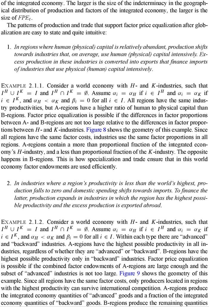
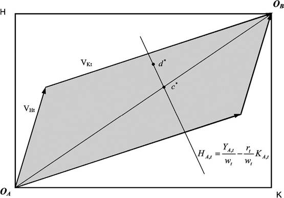
Figure 8. Notes. The box in this figure is a geometrical representation of the set Dt, as each element of this set is a point in the box and vice versa. For instance, d* is a factor distribution such that A-regions have more human and physical capital than B-regions; but human capital is relatively more abundant in A-regions than in B-regions. The box also contains a set of vectors that represent the factor usage per industry that would apply inthe integrated economy. For instance, the vector Vj_t has height Hit and width Kjt ∙ The set FPEt is the gray area. Since all regions have the same industry productivities, production trivially takes place only in regions with the highest possible productivity [requirement (R1)]. Each of the points in the gray area can be generated as a convex combination of the integrated economy’s vectors of factor usage per industry [requirement (R2)]. Since βj = 0, trivially there are no fixed costs of production that are incurred twice [requirement (R3)]. Points outside of the shaded area do not have this property and therefore do not belong to FPEt. The factor content of production is given by the regions’ factor endowments, i.e. d^*. Since all regions have the same spending shares and use the same techniques to produce all goods, the factor content of consumption lies in the diagonal, i.e. c*. In A-regions, the H-industry is a net exporter while the K-industry is a net importer. The opposite occurs in B-regions.

of “backward” goods. This is how specialization and trade ensure that in this world economy production takes place only where industry productivities are higher.

3. Within each industry, only one region produces each input variety and exports it to all other regions. Ifan industry is split among various regions, there is likely to be two-way trade within the same industry³

Example 2.1.3. Consider any of the world economies of the previous examples, but assume now that β_i = 1 for all i ∈ I. Assume d_t ∈ FPE_t. Since the fixed costs of

³¹ I say “likely to be” because a region might produce the final good for domestic use, and import the nec­essary input varieties. It is usual in trade models to set βj = 1 and then drop the “likely to be” from the statement.

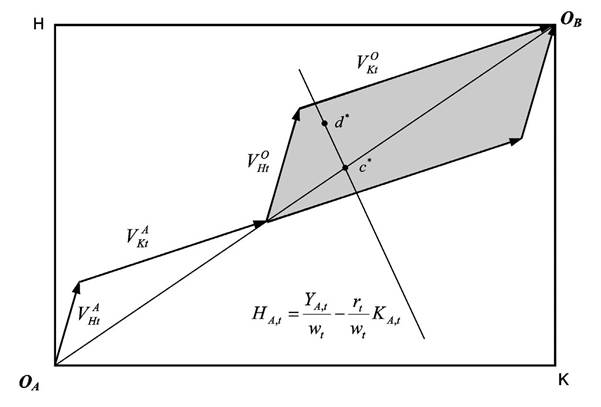
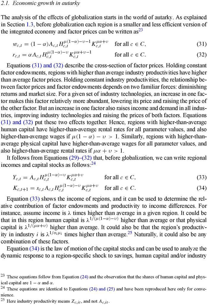
Figure 9. Notes. The box in this figure is a geometrical representation of the set Dt, as each element of this set is a point in the box and vice versa. For instance, d* is a factor distribution such that A-regions have more human and physical capital than B-regions; but human capital is relatively more abundant in A-regions than in B-regions. There are four different industries, “advanced” physical (human) capital intensive and “backward” physical (human) capital intensive. The A-countries have a highest productivity in the “advanced” industries; technologies in the “backward” industries are equal in all countries. The vectors V-X have height hX and width K XX and represent the factor content of the X-industries, where X = A, B stands for “advanced” or “backward” industries. The set FPEt is the shaded area. In this set, all “advanced” industries must be located in the A-countries [requirement (R1)]. Once this requirement is satisfied, each of the points in the shaded area can be generated as a convex combination of the integrated economy’s vectors of factor usage of the “backward” industries [requirement (R2)]. Since β- = 0, trivially there are no fixed costs of production that are incurred twice [requirement (R3)]. Points outside of the shaded area do not have both properties and therefore do not belong to FPEt. The factor content of production is given by the regions’ factor endowments, i.e. d^*. Since all regions have the same spending shares and use the same techniques to produce all goods, the factor content of consumption lies in the diagonal, i.e. c*. In H-regions, the H-industry is a net exporter while the K -industry is a net importer. The opposite occurs in K -regions.

producing inputs contain the cost of building a specialized production plant, all input producers choose to concentrate their production in one region in order not to duplicate these costs. Therefore, each region produces a disjoint set of input varieties. This is how specialization and trade allow the world economy to exploit increasing returns to scale and therefore benefit from a larger market size.

By adopting these patterns of specialization and trade, the world economy is able to reap all the benefits of economic integration without any factor movements. Using the jargon of trade theory, goods trade is a “perfect substitute” for factor movements if d_t ∈ FPE_t. Whenthis is the case, factor prices are given by

The world economy is able to operate at the same level of efficiency as the integrated economy despite the immobility of factors. Equations (31) and (32) showed that, before globalization, cross-regional differences in factor proportions and industry productivi­ties lead to differences in the way industries operate (i.e. their factor proportions and productivity) and also in the size of their markets. Regions with a high ratio of human to physical capital have high wage-rental ratios. Regions with high industry productiv­ities and abundant human and physical capital have high factor prices. But Equations (37) and (38) show that, after globalization (and if d_t ∈ FPE_t), cross-regional differ­ences in factor proportions and industry productivities neither change the way industries operate, nor do they affect the size of their markets. Goods trade allows regions to ab­sorb their differences in factor endowments and industry productivities by specializing in those industries that use their abundant factors and have the highest possible produc­tivity, without the need for having different factor prices. Goods trade also eliminates the effects of regional size on factor prices by creating global markets.

These observations have important implications for the world income distribution and, consequently, for any attempt to determine the relative contribution of factor en­dowments and productivity to income differences. Substituting Equations (37) and (38) into Equation (29), we find that

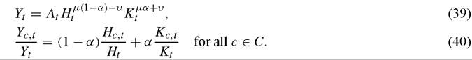
A comparison between these equations and Equation (33) shows that the relative con­tribution of factor endowments and productivity to income differences is fundamentally affected by globalization. Equation (33) differs from Equations (39) and (40) in three important respects: the elasticity of substitution between domestic human and physical capital is one in Equation (33) but infinite in Equations (39) and (40); domestic pro­ductivity appears in Equation (34) but not in Equations (39) and (40); and income is homogeneous of degree μ on domestic factor endowments in Equation (34) but only of degree one in Equation (39) and (40). Each of these differences echoes a different aspect of globalization, and I shall discuss them in turn.

Globalization raises the elasticity of substitution between human and physical capital from one to infinity because structural transformation (a shift towards industries that use the locally abundant factor) replaces factor deepening (forcing industries to use more of the locally abundant factor) as a mechanism to absorb differences in factor proportions. Assume a region has a ratio of human to physical capital λ times higher than average. Before globalization, each of its industries is forced to operate with a ratio of human to physical capital that is λ times average, and this requires a wage-rental ratio that is λ^-1 times average. After globalization, the region simply shifts its production towards in­dustries that are human-capital intensive, keeping the ratio of human to physical capital of its industries constant. This does not require changes in the wage-rental ratio.

Globalization eliminates differences in industry productivities as a source of income differences because structural transformation (a shift towards industries that have high productivity) also replaces productivity deepening (forcing low-productivity industries to produce) as a mechanism to absorb differences in industry productivities. Assume now that a region has average factor endowments but higher than average industry pro­ductivities. For instance, the region’s productivity is λ times higher than the rest of the world in a subset of industries of combined size σ, and equal to the rest of the world in the remaining ones. Before globalization, this productivity advantage allows the region to produce λ^σμ output than average with the same factors, holding constant technology. After globalization, the region takes over all world production of those industries in which its productivity is higher and scales back the rest of its industries. This allows the rest of the world to take full advantage of the region’s high productivity and catch up with it in terms of income (even though not in productivity).

Globalization reduces the effects of factor endowments on relative incomes because it converts regional markets into global ones. Assume now that a region has average industry productivities, but its human and physical capitals are both λ times above av­erage. Before globalization, the region’s higher factor endowments allow it to produce more output than the average region. This effect is further reinforced because the re­gion’s larger market size allows it to have a better technology than average. Therefore, in autarky the region’s income is λ^μ times higher than the world’s average. After glob­alization, this additional market size effect disappears since the relevant market is the world market and this is the same for all regions. Therefore, after globalization the re­gion’s income is only λ times higher than the world average income.

Globalization also influences the dynamics of the world economy. Assume d_t ∈ FPE_t for all t, then it follows from Equations (30), (37) and (38) that

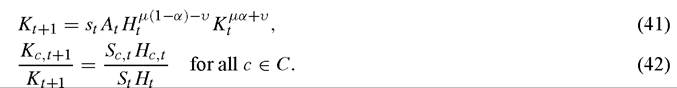
A comparison between these equations and Equation (34) shows how globalization affects the dynamic responses to region-specific shocks. After globalization, positive (and permanent) shocks to savings and human capital still raise a region’s capital stock and income. But now the effects of these shocks spill over to other regions. Shocks to productivity can only affect a region’s income if they push outward the world produc­tivity frontier. And, in this case, all countries equally benefit.^[293]

Another important implication of Equations (39)-(42) is that globalization breaks down the connection between the long run properties of the growth process and the stability of the world income distribution.^[294] Assume again that the joint distribution of

savings, human capital and productivities is stationary. Then, Equation (41) shows that it still is the relative strength of diminishing returns and market size effects that deter­mines whether world average income is stationary or not. But Equation (42) shows that now the world distribution of capital stocks is stationary regardless of parameter values. The same applies to the world income distribution [see Equation (40)]. Therefore, all re­gions share a common growth rate in the long run. The reason is simple: physical capital accumulation in high-savings and high-human capital regions is absorbed by increased production in industries that use physical capital intensively, and this lowers the prices of these industries and increases the prices of industries that use human capital inten­sively. This increases wages and savings in low-savings and low-human capital regions. In a nutshell, movements in goods prices positively transmit growth across regions and ensure the stability of the world income distribution.^[295]

The main feature of the factor-price-equalization world is that diminishing returns and market size effects are global and not local. This observation has important impli­cations for growth theory. Explanations for why the world grows faster today than in the past should feature diminishing returns and market size effects in the lead role, and relegate savings and human capital to a secondary one. But explanations of why some countries grow faster than others should do exactly the opposite, giving the lead role to savings and human capital and relegating diminishing returns and market size effects to a secondary role. A distinctive feature of the integrated economy is therefore a sharp dis­connect between the determinants of average or long run growth and the determinants the dispersion or the cross-section of growth rates.^[296]

The factor-price-equalization world neatly illustrates the potential effects of trade on the world income distribution and its dynamics, and it shows why and how goods trade can be a perfect substitute for factor movements. But the real world has not achieved yet the degree of economic integration that this model implies. One does not need so­phisticated econometrics to conclude that wages vary substantially around the world. It is less obvious but probably true as well that rental rates also vary substantially around the world. These differences in factor prices indicate that regional differences in factor endowments and/or industry productivities are so large that goods trade cannot make up for factor immobility.

What trade always does is to create a global market in which only the most competi­tive producers of the world can survive. Trade forces high-cost industries to close down and offers low-cost industries the opportunity to grow. If d_t ∈ FPE_t all regions contain enough of these low-cost industries to employ all of their factors at common or equal­ized factor prices. But this need not be always the case. If d_t ∈ FPE_t regions with low industry productivities and sizable factor endowments are forced to offer cheap factors to compete, while regions with high industry productivities and small factor endow­ments are able to enjoy expensive factors. These price differences indicate that factors are not deployed where they should and the world economy does not operate efficiently. To study the origins and effects of these world inefficiencies, it is necessary first to review some formal aspects of the model after globalization.

2.3. Formalaspectsofthemodel

As mentioned already, in the absence of asset trade analogues of Equations (1) and (2) apply now to each region of the world economy. A regional analogue to Equation (3) also applies since it is a direct implication of our Cobb-Douglas assumption for the consumption and investment composites. Since all regions share spending patterns and face the same goods prices, the price of consumption and investment is the same for all. We keep this common price as the numeraire and, as a result, Equation (4) also applies. Equations (5)-(6) describing technology apply to all regions, with the corresponding factor prices and industry productivities.

After globalization, Equations (7)-(10) describing pricing policies, input demands and the free-entry condition apply only to those regions that host the lowest-cost pro­ducers of the world. The rest cannot compete in global markets. To formalize this notion, define the following sets of industries:

An industry belongs to I_c,_t if and only if producers located in region c are capable of competing internationally in this industry at date t.^[297] Note that a region can be com­petitive in a given industry because it offers high productivity or a cheap combination of factor prices. The main implication of goods trade is that industries do not locate in regions where they are not competitive,

Since goods markets are integrated, Equation (11) describing market clearing in global goods markets still applies. But now Equations (12) and (13) describing mar­ket clearing in global factor markets must be replaced by analogue conditions imposing

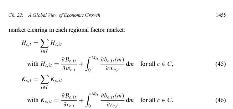
Equations (45)-(46) state that the regional supplies of labor and capital must equal their regional demands. The latter are the sum of their industry demands, and these are calculated by applying Shephard’s lemma to Equations (5) and (6).

This completes the formal description of the model. For any admissible set of capital stocks, i.e. K_c0 for all c ∈ C, and sequences for the vectors of savings, human capital and industry productivities, i.e. S_ct, H_ct and A_cit for all c ∈ C and for all i ∈ I, an equilibrium of the world economy after globalization consists of sequences of prices and quantities such that the equations listed above hold at all dates and states of nature. Although there might be multiple geographical patterns of production and trade that are consistent with world equilibrium, the assumptions made ensure that prices and world aggregates are uniquely determined.^[298]

We are ready now to re-examine the effects of globalization on factor prices and the world income distribution. We have already found that, if d_t ∈ FPE_t globalization elim­inates all regional differences in factor prices and permits the world economy to operate at the same level of efficiency as the integrated economy. In this case, global market forces are strong enough to ensure that diminishing returns and market size effects have a global rather than a regional scope. This is no longer the case if d_t / FPE_t since glob­alization cannot eliminate all regional differences in factor prices. These factor price differences reflect inefficiencies of various sorts in the world economy.

Efficiency requires that factor usage within an industry be the same across regions. This is a direct implication of assuming diminishing returns to each factor in production. The problem, of course, is that regional factor proportions vary. Structural transforma­tion allows regions to accommodate all or part of their differences in factor proportions without factor deepening. If there are enough industries that use different factor propor­tions, factor prices are equalized across regions. If there are not enough industries that use different factor proportions, regions must lower the price of their abundant factor and raise the price of their scarce one to attract enough firms to employ their factor endowments. In this case, industries in different regions use different factor proportions and the world economy is inefficient. Section 2.4 studies the properties of the growth process in this situation.

Efficiency also requires that industries locate in those regions that offer them the highest possible productivity. Structural transformation allows regions to accommodate all or part of their differences in industry productivities without productivity deepening. If all regions have enough industries with the highest productivity, factor prices are equalized across regions. If some regions do not have enough industries with the highest productivity, they are forced to produce in low productivity industries and must lower their factor prices to be able to compete internationally. Section 2.5 shows how this affects the properties of the growth process.

In the presence of these two types of inefficiency, diminishing returns retain a regional scope even after globalization. Regional differences in factor prices still reflect regional differences in factor abundance and industry productivities, although the mapping be­tween these variables is much more subtle than in the world of autarky. However, even in the presence of these inefficiencies regional differences in factor prices cannot reflect regional differences in market size. For market size effects to retain a regional scope after globalization we need to introduce impediments to goods trade. And this task is left for Section 3.

2.4. Limits to structural transformation (I): factor proportions

It follows from Definition (36) that factor prices are equalized if and only if it is possible to achieve full employment of human and physical capital in all regions producing only with the highest productivity [requirement (R1)], with the factor proportions used in the integrated economy [requirement (R2)], and without incurring a fixed cost more than once [requirement (R3)]. Moving away from the factor-price-equalization world means that we must consider the violation of one or more of these requirements. Since the market for each input is “small”, I assume that regions are large enough to ensure that requirement (R3) is always satisfied.^[299] Therefore, in the remainder of this section I will focus on violations of requirements (R1) and (R2). In this subsection, we study the effects on the growth process of violations to requirement (R2), keeping the assumption that requirement (R1) is not binding. This assumption will be removed in Section 2.5.

To formalize the notion that requirement (R1) is not binding, define I*_t as the set of industries in which region c has the highest possible productivity I*_tt ? {i ∈ I | c ∈ argmax_c∕∈_c{Z_c∕,_it}} for all c ∈ C. To ensure that requirement (R1) is not binding in the models of this section, for each of them I first construct the set of “unrestricted” world equilibria by assuming that I* _t = I for all c ∈ C.As mentioned, all these equilibria share the same prices and world aggregates, but might exhibit different geographical patterns of production. In these “unrestricted” world equilibria, some industries might not operate in all regions. Naturally, prices and world aggregates would not be affected if regions did not have the best possible technologies in some or all of the industries in which they do not produce. Therefore, we can trivially relax the assumption that I* _t contains all industries, and instead assume only that there exists an “unrestricted” equilibrium such that, for all c ∈ C, the industries not included in I* _t do not operate in the region. This defines the extent to which regional differences in industry produc­tivities are allowed in this section. It follows that requirement (R1) is never binding and comparative advantage is determined solely by regional differences in factor propor­tions.

In the worlds we consider in this subsection it is not possible in general to employ all factors in all regions using the techniques of the integrated economy. Even if they concentrate all of their production in industries that use human capital intensively, re­gions with abundant human capital might lack enough physical capital to produce with the factor proportions that these industries would use in the integrated economy. These regions are therefore forced to use a higher proportion of human capital in their in­dustries and this requires them to have a lower wage-rental ratio than in the integrated economy. Naturally, the exact opposite occurs in regions with abundant physical capi­tal. This situation can be aptly described as a geographical mismatch between different factor endowments.

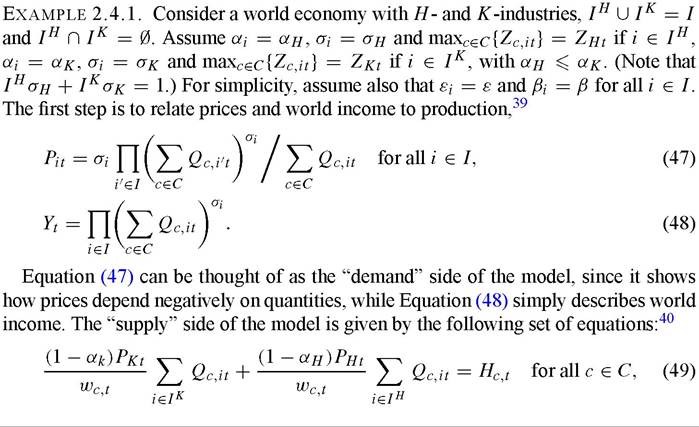
To study the causes and effects of this mismatch, I present two examples that help build intuitions that apply more generally. The first example is the two-industry case that is so popular in trade theory:

^[1] These equations follow from Equations (3) and (4).

^[1] Equations (49) and (50) follow from Equations (45) and (46), while Equations (51) and (52) follow from Equations (7) and (9) after using Equation (17) to eliminate the number of input varieties.

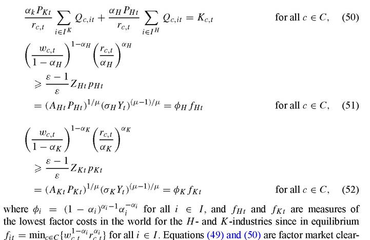
ιng conditions, while Equations (51) and (52) are just a transformation of the pricing equations of each industry (for both final goods and intermediate inputs). Naturally, these pricing equations hold with strict equality if there is positive production in the corresponding industry. Equations (49)-(52) determine the production of each type of industry and the factor prices of region c, as a function of world prices and income.^[300]

Equations (47)-(52) determine prices and quantities as a function of the distribution of factor endowments. Together with the regional analogues to Equation (1), the initial condition and the dynamics of the exogenous state variables, these equations provide a complete characterization of the world equilibrium. Next, I describe some its most salient features.

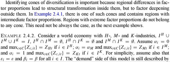
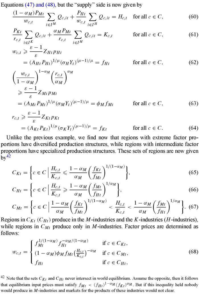
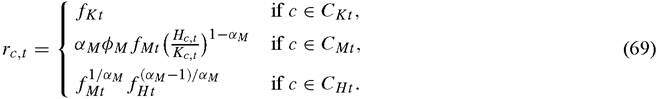
Regions with extreme factor proportions have specialized production structures, while regions with intermediate factor proportions have diversified production struc­tures. Let C_Kt (C_Ht) be the set of regions where there is production only in K -industries (H-industries), and let C_Mt be the set of regions where there is production in both types of industries. In fact, it follows from Equations (49)-(52) that these sets of regions are defined as follows:

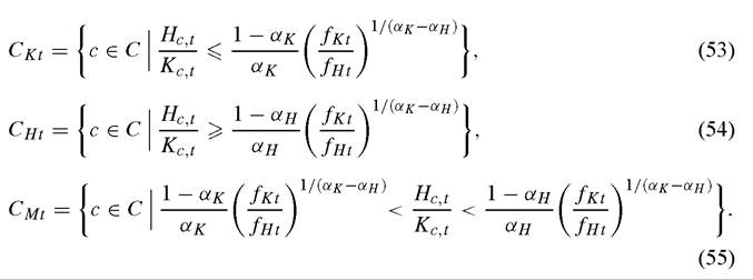
It follows from Equations (51) and (52) that factor prices are the same for all c ∈ C_m. If the dispersion in regional factor proportions is not too large, and the dispersion in fac­tor intensities is not too low, C_κt = C_Ht = 0 and there is factor price equalization. Oth­erwise, this world economy exhibits a limited version of the factor-price-equalization result since factor prices are still equalized for all c ∈ C_Mt. It is common in trade theory to refer to a group of regions that share the same factor prices as a “cone of diversifi­cation”. In fact, we can write the wage and the rental as a function of f_Ht and f_κt as follows:

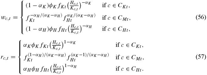
The wage is continuous and weakly declining on the human to physical capital ratio, while the rental is also continuous but increasing on this same ratio. The most note­worthy feature of these relationships is that they exhibit a “flat” for the set of human to physical capital ratios that define the cone of diversification. The top panel of Fig­ure 10 shows how the wage-rental ratio varies with a region’s ratio of human to physical capital. Regional differences in this ratio reflect factor abundance in the usual way. In regions with a high (low) ratio of human to physical capital the price of human capital is low (high) relative to physical capital. Factor prices do not reflect however regional differences in industry productivities and/or market size.

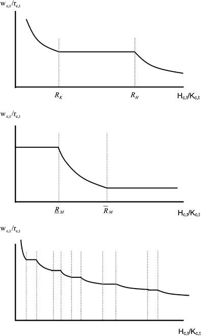
Figure 10. Notes. This figure shows how the wage-rental ratio varies with the factor proportions. The top panel represents a two-goods, one-cone world where countries with extreme factor proportions are outside the cone (Example 2.4.1). The middle panel represents a three-good, two-cone world where countries with intermediate factor proportions lie outside the cone (Example 2.4.2). The bottom panel shows a world with multiple goods and cones.

It is now straightforward to compute the world income distribution as a function of ^fHt ^{and f}Kt^,

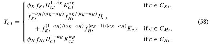
We can use Equation (58) to re-evaluate earlier results about the relative contribution of factor endowments and industry productivities to income differences across regions. The first result is that the elasticity of substitution between human and physical capital is one outside the cone of diversification, but infinity within the cone. This elastic­ity reflects the relative importance of structural transformation and factor deepening as means to absorb regional differences in factor proportions. The second result is that re­gional differences in industry productivities continue not playing a role in determining regional income differences. This, of course, is not surprising given the assumption we have made about requirement (R1) not being binding. The third and final result is that relative incomes are homogeneous of degree one on factor endowments. This not sur­prising either since it simply confirms the absence of market size effects at the regional level.

We can also write the dynamics of the capital stock as a function of f_Ht and f_κt,

270" class="lazyload" data-src="/files/uch_group77/uch_pgroup302/uch_uch7199/image/image270.jpg">

The specific dynamics of this example are hard to determine, since f_Ht and f_κt change from generation to generation. It is easy to construct examples in which the world economy moves towards factor-price equalization; examples in which the world economy moves away from factor-price equalization; or examples in which the world economy alternates between periods in which factor prices are equalized and periods in which they are not. These dynamics depend on all the parameters the model (including initial condition) and the evolution of the exogenous state variables, i.e. savings, hu­man capital and industry productivities. Regardless of the specific dynamics, the world income distribution is stable if the joint distribution of these variables is stationary. Eco­nomic growth is positively transmitted across regions through changes in goods prices. This stabilizing role of trade is further reinforced by the fact that regions outside the cones cannot absorb capital accumulation through structural transformation and, conse­quently, experience diminishing returns in production.

Once again, the wage is continuous and weakly declining on the human to physical capital ratio, while the rental is also continuous but increasing on this same ratio. But now these relationships exhibit at most two “flats”, one for each set of human to physical capital ratios that defines a cone of diversification. Regional differences in factor prices reflect again factor abundance in the usual way. This world economy contains at most two cones of diversification.^[301] Regions with extreme factor proportions belong to one of them, while regions with intermediate factor proportions do not. The middle panel of Figure 10 shows how the wage-rental varies with a region’s ratio of human to physical capital.

It is straightforward to compute the analogues of Equations (58) and (59) for this example and check that the mapping from factor endowments to incomes and capital accumulation is also linear within the cones and takes the Cobb-Douglas form outside of them. The picture of the growth process that comes out of this example is therefore very similar to the on in Example 2.4.1.

Examples 2.4.1 and 2.4.2 can be generalized by introducing further industries with different factor intensities. As we do so, the potential number of cones increases. But the overall picture remains the same. The world economy sorts itself out in a series of cones of diversification. The bottom panel of Figure 10 depicts a case with multiple cones of diversification.^[302] Small regional differences in factor proportions lead to struc­tural transformation within cones, but to factor deepening outside them. Large regional differences in factor proportions might span one or more cones and therefore lead to a mix of structural transformation and factor deepening. Therefore, the world of diver­sification cones can be seen as being somewhere in between the world of factor-price equalization and the world of autarky.^[303]

In the light of these results, we must slightly revise our earlier discussion of the effects of globalization on the source of income differences. As in the world of factor­price equalization, differences in domestic productivities cannot be a source of income differences and relative incomes are homogeneous of degree one with respect to factor endowments. But unlike the world of factor-price equalization, the elasticity of substitu­tion between domestic factors is no longer infinity but instead lies somewhere between one (outside cones) and infinity (within cones). As mentioned, this elasticity measures the relative importance of structural transformation and factor deepening as a means to accommodate regional differences in factor proportions. And this relative importance in turn depends on various factors, most notably how dispersed are factor intensities across industries. Two extreme examples make this point forcefully. If the dispersion in industry factor intensities is extreme, i.e. α_i ∈ {0, 1} for all i ∈ I, then regional differences in factor proportions always lead to structural transformation and the world income distribution is given by Equations (39) and (40).^[304] If the dispersion in industry factor intensities is instead negligible, i.e. α_i = α for all i ∈ I, then regional differences in factor proportions always lead to factor deepening and the world income distribution is given by^[305]

As in the world of autarky, the elasticity of substitution across factors is one [see Equation (33)]. But unlike the world of autarky, regional differences in industry pro­ductivities and market size play no role in explaining regional income differences.

We do not need to revise however our earlier discussion of how globalization af­fects the dynamic responses to region-specific shocks. In this respect, the world with diversification cones offers the same insights as the world of factor-price equalization. Region-specific shocks to savings and human capital have positive effects that spill over to other regions, while shocks to industry productivities only have effects if they push outwards the world productivity frontier. Economic growth is positively transmit­ted across regions through changes in goods prices and this keeps the world income distribution stable. In fact, this force towards stability is further reinforced in regions that are outside a cone by the existence of diminishing returns in production.

We conclude therefore that violations to requirement (R2) do not alter much the picture came out of the factor-price-equalization world. Surely the geographical mis­match between different factor endowments implied by these violations might generate large inefficiencies that, in turn, might lead to sizable regional differences in factor prices. Therefore, there might be important quantitative differences between a world with many diversification cones and the world of factor-price-equalization. But the qual­itative properties of the growth process of these two worlds remain relatively close to each other, and far away from those of the world of autarky.

2.5. Limits to structural transformation (II): industry productivities

Consider next worlds where requirement (R1) is either binding or fails. Regions with few high-productivity industries might find that even if they concentrate all of their production in those industries, they cannot employ all of their factors and produce the same quantities as the integrated economy. These regions are therefore forced to ex­ceed the production of the integrated economy in those industries and/or move into low-productivity industries. Whatever the case, this requires these regions to offer low factor prices to employ all of their factors. This situation can be aptly described as a geographical mismatch between industry productivities and factor endowments.

To make further progress, it is necessary to be more explicit about why and how industry productivities differ across regions. The first example considers the case in which regional differences in productivities take the popular factor-augmenting form:

48 Take, for instance, the case of two regions and two industries. If one region has the highest productivity in both industries the only factor distribution that leads to factor-price equalization is the one in which all factors are located in this region. If instead each region has the highest productivity in a different industry, the only factor distribution that leads to factor-price equalization is the one in which each region receives the exact quantity of factors that its high-productivity industry uses in the integrated economy.

49 The re-normalized model is a bit less general than the model of the previous section since it does not display regional differences in industry productivities. We could (trivially) generalize this example to allow for regional differences in industry productivities, but keeping the assumption that requirement (R1) is not binding in the re-normalized model.

50 For instance, Equations (56) and (57) describe the productivity-adjusted factor if we further assume that the world economy contains two types of industries as in Example 2.4.1. Similarly, Equations (68) and (69) describe productivity-adjusted factor prices if we instead assume thatthe world economy contains three types of industries as in Example 2.4.2.

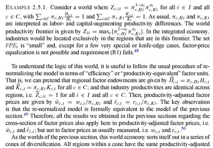
factor prices, although possibly different factor prices as usually measured. Regional differences in productivity-adjusted factor proportions lead to structural transformation within cones, and to factor deepening across them. When all regions are located within a single cone, we have the conditional factor-price-equalization result emphasized by Trefler (1993). That is, regional differences in factor prices reflect only differences in factor-augmenting productivities and are not related to differences in productivity- adjusted factor proportions.

Although the presence of factor-augmenting productivity differences does not alter much the formal or mathematical structure of the model, it has important implica­tions for the question of why some regions are richer than others. Unlike the worlds of Section 2.4, we now have that productivity differences become a source of income differences across countries. For instance, if all regions belong to a single cone of diver­sification we have the following counterpart to Equation (40),

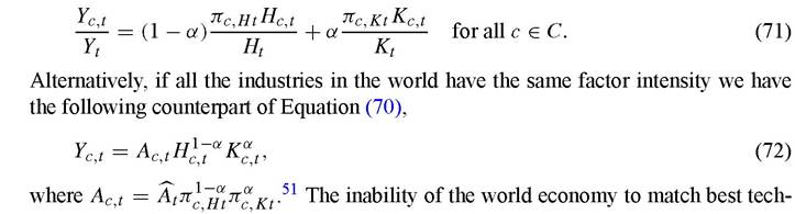
nologies with appropriate factors moves us a step closer to the world of autarky, since regional productivities now affect regional incomes. Moreover, since now the world op­erates below its productivity frontier shocks to regional factor productivities have effects even if they do not push this frontier. Note however that, as in the worlds of Section 2.4, the elasticity of substitution between domestic factors still lies somewhere between one (outside cones) and infinity (within cones); and relative incomes are homogeneous of degree one with factor endowments.

The rest of the picture of the growth process that comes out of this world remains close to the world of factor-price equalization. Region-specific shocks to savings and human capital have positive effects that spill over to other regions. Economic growth is positively transmitted across regions through goods prices and this keeps the world income distribution stable. If the conditional version of the factor-price-equalization theorem does not hold, regions outside the cones experience diminishing returns and this reinforces the effects of changes in product prices on the stability of the world income distribution.

Assuming that regional productivity differences take the factor-augmenting form discussed in Example 2.5.1 is popular because it yields tractable models. But the factor­augmenting view of productivity differences hides some interesting effects of trade on

51 This model therefore provides an alternative theoretical foundation for the work of Mankiw, Romer and Weil (1992), Hall and Jones (1999) and Klenow and Rodriguez-Clare (1997). the world income distribution and its stability. One reason is that, in the world of factor­augmenting productivity differences, comparative advantage is still determined solely by regional differences in factor proportions, albeit productivity-adjusted ones. The next example provides a dramatic illustration of how regional differences in industry produc­tivities could determine comparative advantage, and how this brings about a new effect of trade on the world income distribution:

cations and goods prices, while Equations (74) and (75) provide the equilibrium factor allocations as a function of aggregate factor endowments. By substituting Equations (74) and (75) into Equation (73), we obtain the world income distribution as a function of factor endowments and input prices.⁵² It is immediate to show that the elasticity of substitution between human and physical capital is between one and infinity; that re-

52 This relationship is formally analogous, for instance, to Equation (58) in Example 2.4.1. gional differences in industry productivities affect regional differences in income; and that the world income distribution is homogeneous of degree one with respect to factor endowments.

These results are obtained from a relationship between incomes, factor endowments and industry productivities that holds constant input prices. Once we substitute input prices into this relationship, we find that the world income distribution is given by

Equation (76) states that the share of world income of each region equals that share of world spending on the industries located in the region, and it does not depend on domestic factor endowments. What is going on? Assume a region has a ratio of human to physical capital λ times higher than average. Since the region is producing a fixed set of goods, it is forced to operate with a ratio that is λ times higher than average, and this requires a wage-rental ratio that is λ^-1 higher than average. Therefore the elasticity of substitution between human and physical capital in production is one. What is different here is that relative incomes are now homogeneous of degree zero with respect to factor endowments. Assume a region’s human and physical capitals are both λ times average. Since production is homogeneous of degree one with factor endowments, its production of all industries is λ times average. But since the country faces a demand for its products with price-elasticity equal to one, the prices of its products are λ^-1 times average. As a result, the income of the region is just average, despite its factor endowments being λ times average.

So what should we conclude about the degree of homogeneity of relative incomes with respect to factor endowments? As Equations (73)-(75) and (76) show, in empirical applications it will depend on whether we are holding goods prices constant or not. If we are holding these prices constant, then relative incomes are homogeneous of degree one in factor endowments. If we are not holding goods prices constant, then the degree of ho­mogeneity of relative incomes with respect of factor endowments lies between zero and one. In this example, this degree of homogeneity is zero because regional differences in factor endowments are absorbed by regional variation in the quantities produced of each input. In Examples 2.4.1, 2.4.2 and 2.5.1, this degree of homogeneity was one be­cause regional differences in factor endowments were absorbed by regional variation in the number of input varieties produced. The next example, inspired by Dornbusch, Fischer and Samuelson (1977), neatly clarifies this point by showing an intermediate world where both margins are at work.

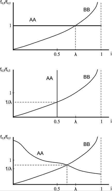
Example 2.5.3. Consider a world with two regions C = {N, S}, and a continuum of industries I = [0, 1]. Assume all industries have the same factor intensity, α_i = α for all i ∈ I. For simplicity, let also ε_i = ε and β_i = β for all i ∈ I.It follows immediately that^{[306] [307] [308]}

Having already found the pattern of production and trade (i *) and relative factor costs (∕n, t/fs, _t), Equation (80) can then be used to determine absolute factor costs.

This world is somewhat different form the ones we have seen so far in that we have only two regions. To think about the effects of factor endowments on relative incomes, I consider next a situation in which both regions have symmetric technologies and differ in that North’s factor endowments are λ (> 1) times larger than South’s.^[309] Figure 11 depicts this world. The AA and BB lines represent Equations (78) and (79), respectively. The AA line is nonincreasing because T_i is nonincreasing in i, while the BB line is nondecreasing because X_i is nondecreasing in i. The existence of a unique crossing point follows since the BB line takes value zero at i = 0 and slopes upward towards infinity at i = 1.

The top panel of Figure 11 shows the case in which T_i is flat. This case corresponds to a world in which differences in industry productivities are minimal or irrelevant at the margin as in Examples 2.4.1, 2.4.2 and 2.5.1. This allows Northto employ its larger factor endowments by producing a larger number of varieties than South. Factor costs are the same in both regions and, as a result, North’s income is λ times South’s. Relative incomes (after substituting in goods prices) are homogeneous of degree one on factor endowments.

The middle panel of Figure 11 shows the opposite case in which Ti is vertical. This case corresponds to a world in which differences in industry productivities are extreme as in Examples 2.5.2. North is forced to employ its larger factor endowments by produc­ing a higher quantity of each of its varieties. Factor costs in North are λ^-1 times those of South and, as a result, North’s income equals that of South. Relative incomes (after substituting in goods prices) are homogeneous of degree zero on factor endowments.

The bottom panel shows the intermediate case in which T_i is neither flat nor vertical. Since the slope reflects how strong are differences in industry productivities, we are somewhere in between the two extreme examples considered up to now. North employs its larger factor endowments by producing a larger number of varieties and also a larger quantity of each of them. Factor costs in North are somewhere between λ^-1 and one times those of South. The degree of homogeneity of relative incomes (after substituting in goods prices) on factor endowments is therefore somewhere between zero and one.

It is possible to generalize Example 2.5.3 in a variety of directions. For instance, one could allow for industry variation in factor intensities and many regions.^[310] This is important in empirical applications, of course. But the central message remains. The effects of factor endowments on relative incomes depend on regional differences in industry productivities. If these differences are small, regions with larger factor endow­ments absorb them mostly through structural transformation: not changing much their

Figure 11. Notes. This figure shows how pattern of production and trade (i*) and relative factor costs (fN,t/fs,t) are determined in Example 2.5.3. The top panel shows the case of arbitrarily small differences in industry productivities. The middle panel shows the case of arbitrarily large differences in industry produc­tivities. The bottom panel shows the intermediate case.

production in existing industries and moving into new industries where the region's productivity relative to the rest of the world is similar to existing ones. If differences in industry productivities are large, regions with larger factor endowments absorb them by productivity deepening: substantially increasing their production in existing industries and/or moving into industries where the region's productivity relative to the rest of the world is substantially lower than in existing ones.

One can conclude from this discussion that differences in industry productivities cre­ate another force for diminishing returns to physical capital accumulation. As physical capital is accumulated, quantities produced increase and the terms of trade worsen. The result is a reduction in factor prices that lowers wages, savings and capital accumula­tion. This is a central aspect of the growth process in a world of interdependent regions generates a force towards the stability of the world income distribution.^[311]

I argued at the end of Section 1 that, if globalization leads to the integrated economy, there is a powerful prescription for economic development: open up and integrate into the world economy. This allows regions to benefit from higher productivity, improved factor allocation and increased market size. Not much has changed here. Naturally, if factor prices are equalized the effects are literally the same as in Section 1 since then globalization leads to the integrated economy. If factor prices are not equalized, the world economy operates with a lower productivity and a worse factor allocation than the integrated economy. This also means that the size of the world economy will be smaller than that of the integrated economy. As a result, all the benefits from globalization are smaller in the worlds of Sections 2.4 and 2.5 than in the world of factor-price equaliza­tion. But it is still relatively straightforward to see that coupled with an appropriate transfer scheme globalization constitutes a Pareto improvement for the world econ­omy. Moreover, since all regions gain from trade there exist Pareto-improving transfer schemes that do not require inter-regional transfers.^[312] Therefore, the prescription for development remains the same: open up and integrate into the world economy.

We have traveled much already, and the global view of economic growth is starting to take shape. This view is more realistic and rich in details than the views that came out from either the world of autarky or the integrated economy. Despite this progress, we should not rest here yet. We have assumed so far that globalization eliminates all impediments to goods trade. This is obviously an unrealistic assumption. Is it also a crucial one?

3.