Trade, Specialization and the World Income Distribution

In this section, I will present a model of the world economy in which countries trade intermediate goods, but trade will have Ricardian features. In particular, each country will specialize in the production of a subset of the available goods in the world economy and will therefore affect the prices of the goods that it supplies to the rest of the world.

The model economy presented here builds on Acemoglu and Ventura (2002). I will start with a simplified version of this model, which features physical capital as the only factor of production. I will then present the full model in which both physical capital and labor are used to produce consumption and investment goods.

In addition to the nature of trade (Heckscher-Ohlin versus Ricardian), another major difference between the model in this section and the previous one will be that now, as in Section 18.3 in the previous chapter, the world economy will exhibit endogenous growth, with the growth rate determined by the investment decisions of all countries. Despite endogenous growth at the world level, international trade (without any technological spillovers) will create sufficient interactions to ensure a common long-run growth rate for all countries. Therefore, the current model will show how international trade, like technological spillovers, will create a powerful force limiting the extent to which divergence can occur across countries.

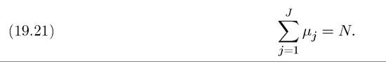
19.4.1. Basics. We consider a world economy consisting of a large number J of “small” countries, again indexed by j = 1,...,J.

Countries differ in their technology, savings and economic policies. For example, country j will be defined by its characteristics (μj,ρj,ζj), where μ is an indicator of how advanced the technology of the country is, ρ is its rate of time preference, and ζ is a measure the effect of policies and institutions on the incentives to invest. All of these characteristics potentially very across countries, but are constant over time. We take their distribution across countries as given. In addition, we assume that each country has a population normalized to 1 and there is no population growth.

All countries admit a representative household with utility function:

where Cj (t) is consumption of country j date t. Preferences are logarithmic and thus more specialized than the typical CRRA preferences we have used so far (for example, in terms of the preferences in (19.1), they involve θ → 1). Logarithmic preferences enable us to simplify the exposition without any substantive loss of generality. On the other hand, the preferences in (19.19) are significantly more flexible than those in the previous section because they allow the discount rates, theto differ across countries. We also assume that country j starts with a capital stock of Kj (0) > 0 at time t = 0.

The budget constraint of the representative household in country j at time t is

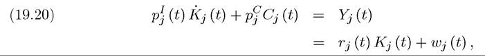
where pj and pj are the prices of the investment and consumption goods in country j (in terms of the numeraire, which will be the ideal price index of traded intermediates; see below).

As noted above, our focus here is with Ricardian models which feature specialization. We will introduce specialization in the simplest possible way. In particular, we will assume that the N intermediates available in the world economy are partitioned across the J countries, such that each intermediate can only be produced by one country. This assumption, which is often referred to as the Armington preferences or technology in the international trade literature, ensures that while each country is small in import markets, it will affect its own terms of trades by the amount of the goods it exports. Denoting the measure of goods produced by country j by μj, our assumption implies that

This equation immediately implies that a higher level of μj implies that country j has the technology to produce a larger variety of intermediates, so we interpret μ as an indicator of how advanced the technology of the country is.

Moreover, let us assume that in each country the production technology of intermediates is such that one unit of capital produces one unit of any of the intermediates that the country is capable of producing and that there is free entry to the production of intermediates. This assumption immediately implies that the prices of all intermediates produced in country j at 772

time t are given by

where recall that rj (t) is the rental rate of return in country j at time t.

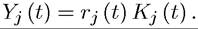
19.4.2. The AK Model. Before presenting the full model, it is convenient to start with a simplified version, where capital is the only factor of production. Consequently, in terms of equation (19.20), we have Wj (t) = 0, and

We assume that both consumption and investment goods are produced using domestic capital as well as a bundle of all the intermediate goods in the world (which are all traded freely). In particular, the production function for consumption goods in country j is:

A number of features are worth noting. First, Kj denotes domestic capital used in the consumption goods sector and enters the production function with exponent 1 — τ. Intuitively, this term corresponds to the services of the domestic capital stock used in the production of consumption goods. It represents the “non-traded” component of the production process, which depends on the services provided by non-traded goods using the capital available in the country. In particular, since there is no international trade in assets, it must be the domestic capital stock that is used in providing these non-traded services, and if a country has a relatively low capital stock, the relative price of capital will be high and less of it will be used in producing consumption goods (and investment goods; see below).

which avoids the counterfactual and counterintuitive pattern of “immiserizing growth” (see Exercise 19.21). The use of constant elasticity of substitution aggregates is familiar by now and plays the same role here as in other models we have seen so far, and enables us to have tractable structure. The expression also makes it clear that there is a continuum N of intermediates (given by equation (19.21) above). Notice that this CES aggregator has an exponent τ, which ensures that the production function for consumption goods exhibits constant returns to scale. The parameter τ is not only the elasticity of the production function of consumption goods with respect to traded intermediates, but it will also be the share of trade in GDP for all countries in this world economy (see Exercise 19.13). Finally, χ is a constant introduced for normalization (see Exercise 19.11).

The production function for investment goods in country j is:

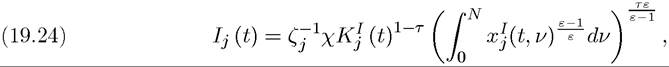
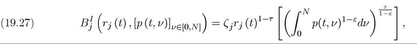
which is identical to that for consumption goods, except for the presence of the term ζj. This allows differential levels of productivity, due to technology or policy, in the production of investment goods across countries. The assumption that these differences are in the in­vestment good sector rather than in the production of consumption goods is consistent with results on the relative prices of investment goods discussed previously, which suggested that in poorer economies investment goods are relatively more expensive.

Market clearing for capital naturally requires

wherecapital used in the production of intermediates and Kj (t) is the total capital stock of country j at time t.

The reader can also see why we have referred to this model as the AK version; the production of both consumption and investment goods uses capital and intermediates that are directly produced from capital. Thus a doubling of the world capital stock will double the output of all intermediates and of consumption and investment goods.

While we can directly work with the production functions for consumption and investment goods, (19.23) and (19.24), as in many trade models, it is simpler to work with unit cost functions, which express the cost of producing one unit of consumption and investment goods in terms of the numeraire (which will be chosen as the ideal price index for intermediates, see equation (19.31) below). Exercise 19.11 shows that the production functions (19.23) and (19.24) are equivalent to the unit cost functions for consumption and production given by

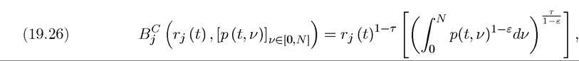
where p(t,ν) is the price of the intermediate ν at time t and the constant χ in (19.23) and (19.24) is chosen appropriately (see Exercise 19.11). Notice that these prices are not indexed by j, since there is free trade in intermediates and thus all countries face the same intermediate prices. The specification using the unit cost functions simplifies the analysis.

A world equilibrium is defined in the usual fashion, as a sequence of prices, capital stock levels and consumption levels for each country, such that all markets clear and the representative household in each country maximizes his utility given the price sequences. Namely, an equilibrium is represented by

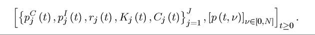
Notice that while the prices of consumption and investment goods and the return to capital are country specific, the prices of intermediates are not. A steady-state world equilibrium is also defined in the usual fashion, in particular, requiring that all prices are constant (as before, this “steady-state” equilibrium will involve balanced growth).

The characterization of the world equilibrium in this case is made relatively simple by the AK technology (and the logarithmic preferences). In particular, the maximization of the representative household, that is, the maximization of (19.19) subject to (19.20) for each j yields the following first-order conditions for each j and t, and the transversality condition: for each j (see Exercise 19.12).

Equation (19.28) is the Euler equation. This equation might first appear slightly different from the standard Euler equations we have encountered throughout the book, but the reader will see that it is identical to the Euler equations implied by the two-sector model in Section 11.3 in Chapter 11 (recall, in particular, equation (11.31)). The difference from the standard Euler equations stems from the fact that we now have potentially different technologies for producing consumption and investment goods, thus individuals that delay consumption have to take into account the change in the relative price of consumption versus investment goods— which explains the presence of the term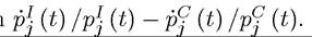In this light, it is clear

that this equation simply requires the (net) rate of return to capital to be equal to the rate of time preference plus the slope of the consumption path.

Equation (19.29) is the transversality condition. Integrating the budget constraint and using the Euler and transversality conditions, we obtain a particularly simple consumption function in this case:

which can be interpreted as individuals spending a fraction ρj of their wealth on consumption at every instant (recall that in this simplified model, there is no labor income and is consumer wealth at current prices).

Our analysis so far has therefore characterized the prices of intermediates and the behavior of the consumption and capital stock for each country. We next need to determine the prices of consumption and investment goods and the relative prices of intermediates in the world economy. As a first step towards this, we define the numeraire for this world economy as the ideal price index for the basket of all the (traded) intermediates. Since the intermediates always appear in the CES form, the corresponding ideal price index is simply

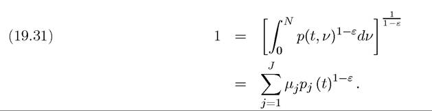
Here the first term defines the ideal price index, while the second uses the fact that country j produces μj intermediates, and each of these intermediates have the same price pj (t) = rj (t) as given by (19.22) above.

This choice of numeraire has another convenient implication. Our assumption that each country is small implies that each exports practically all of its production of intermediates and imports the ideal basket of intermediates from the world economy. Consequently, pj (t) = rj (t) is not only the price of intermediates produced by country j, but also its terms of trade —defined as the price of the exports of a country divided by the price of its imports.

Next, using the price normalization in (19.31), (19.26) and (19.27) imply that the equi­librium prices of consumption and investment goods in country j at time t are given by

This completes the characterization of all the prices in terms of the rate of return to capital. To compute the rate of return to capital, we need to impose market clearing for capital in each country. In addition, we also have a trade balance equation for each country. However, by Walras’ law, one of these equations is redundant. It turns out to be more convenient to use the trade balance equation, which can be written as

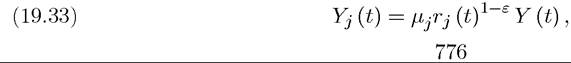
whereis total world income at time t. To see why this equation ensures

balanced trade, note that each country spends a fraction τ of its income on intermediates, and since each country is small, this implies a fraction τ of its income being spent on imports. At the same time, the rest of the world spends a fraction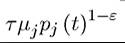of its total income

on intermediates produced by country j (this follows because of the CES aggregator over intermediates combined with the observations that pj (t) is the relative price of each country j intermediate and there are μj of them). Noting that total world income is Y (t) and that Pj (t) ^{= r}j (t), we obtain (19.33). Exercise 19.13 asks you to derive this equation from the capital market clearing equation, (19.25), thus verifying the use of the Walras’ law.

The equations derived so far, in particular (19.22), (19.30), (19.32) and (19.33) together with the resource constraint, (19.20), characterize the world equilibrium fully.

Let us start by describing the state of the world economy, which can simply be represented by the distribution of capital stocks across the J economies (these are the only endogenous state variables). Their law of motion is obtained simply by combining (19.20), (19.30) and

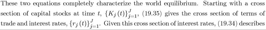
(19.32) on the one hand, and (19.20) and (19.33) on the other. In particular, for each j and t, the law of motion of the capital stock is described by the following pair of differential equations:

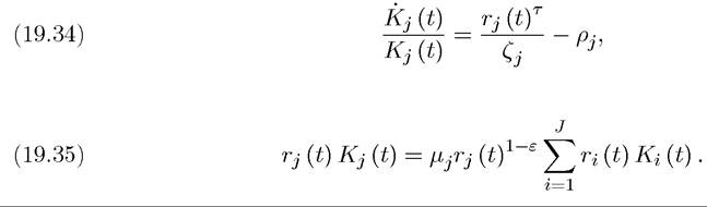
exactly how the cross section of capital stocks will evolve.

The simplicity of these laws of motion are noteworthy. The first, (19.34), determines the evolution of the capital stock of each country simply as a function of their own parameters, ζj, the distortions on the investment good producing sector, and Pj, the discount rate, as well as the equilibrium rental rate. The second, (19.35), expresses the rental rate for each country as a function of the rental rates and capital stocks of other countries.

These two equations immediately establish the following important result:

Proposition 19.10. There exists a unique steady-state world equilibrium where we have

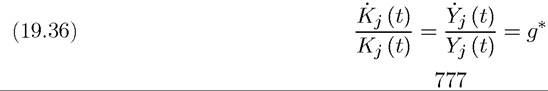
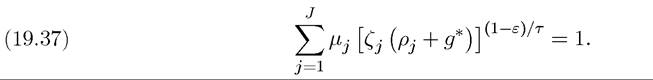
for j = 1,...,J, and the world steady-state growth rate g* is the unique solution to equation

The steady-state rental rate of capital and the terms of trade in country j are given by

This unique steady-state equilibrium is globally saddle-path stable.

Proof. (Sketch) By definition, a steady-state equilibrium must have constant prices, thus a constantThis implies that in any state state, for each must grow at some constant rate g_j. Suppose these rates are not equal for two countries j andTaking the ratio of equation (19.35) for these two countries yields a contradiction, establishing thatis constant for all countries. Equation (19.33) then implies

that all countries also grow at this common rate, say g*. Given this common growth rate,

(19.34) immediately implies (19.38). Substituting this back into (19.35) gives (19.37). Since these equations are all uniquely determined and (19.37) is strictly decreasing in g*, thus has a unique solution, the steady-state world equilibrium is unique.

To establish global stability, it suffices to note that (19.35) implies that rj (t) is decreasing in Kj (t). Thus whenever a country has a high capital stock relative to the world, it has a lower rate of return on capital, which from (19.34) slows down the process of capital accumulation in that country. This process ensures that the world economy, and all economies, move towards the unique steady-state world equilibrium. Exercise 19.14 asks you to provide a formal proof of stability. ?

The results summarized in this proposition are quite remarkable. First, despite the high degree of interaction among the various economies, there exists a unique globally stable steady-state world equilibrium. Second, this equilibrium takes a relatively simple form. Third and most important, in this equilibrium all countries grow at the same rate g*. This third feature is quite surprising, since each economy has access to a AK technology, thus without any international trade, each country would grow at a different rate (for example, those with would have higher long-run growth rates). The process of international trade acts as a powerful force keeping countries together, ensuring that in the long run they will all grow at the same rate. In other words, international trade, together with specialization, leads to a stable world income distribution.

Why is this? The answer is related to the terms of trade effects encapsulated in equation

(19.35). To understand the implications of this equation, considered the special case where

all countries have the same technology parameter, i.e., μj = μ for all j. Suppose also that a particular country, say country j, has lowerand ρj than the rest of the world. Then

(19.34) implies that this country will tend to accumulate more capital than others. But

(19.35) makes it clear that this cannot go on forever and country j, by virtue of being richer than the world average, will also have a lower rate of return on capital. This lower rate of return will ultimately compensate the greater incentive to accumulate in country j, so that capital accumulation in this country converges to the same rate as in the rest of the world.

Intuitively, while each country is “small” relative to the world, it has market power in the goods that it supplies to the world. When it exports more of a particular good, the price of that good declines, so that world consumers should wish to consume the greater amount of this good that is being supplied in the world market. This implies that when a country accumulates faster than the rest of the world, and thus increases the supply of its exports relative to the supplies of other countries exports, it will face worsening terms of trades. This negative terms of trade effect will reduce the income of the country that is accumulating faster. However, more important than this level effect is the dynamic effects of the changes in terms of trades. Recall that equation (19.22) links the rate of return to capital to the terms of trade faced by the country. When a country experiences a worsening in its terms of trade, it also experiences a decline in the rate of return the capital and in the interest rate that the households face. This slows down its rate of capital accumulation, ensuring that in the steady state equilibrium all countries accumulate and grow at the same rate. Therefore, this model shows how pure trade linkages are sufficient to ensure that countries that would otherwise grow at different rates pull each other towards a common growth rate and the result is a stable world income distribution. Naturally, growth at a common rate does not imply that countries with different characteristics will have the same level of income. Exactly as in models of technological interdependences in the previous chapter, countries with better characteristics (higher μ^ and lower ζj and ρj) will grow at the same rate as the rest of the world, but will be richer than other countries. This is most clearly shown by the following equation, which summarizes the world income distribution.

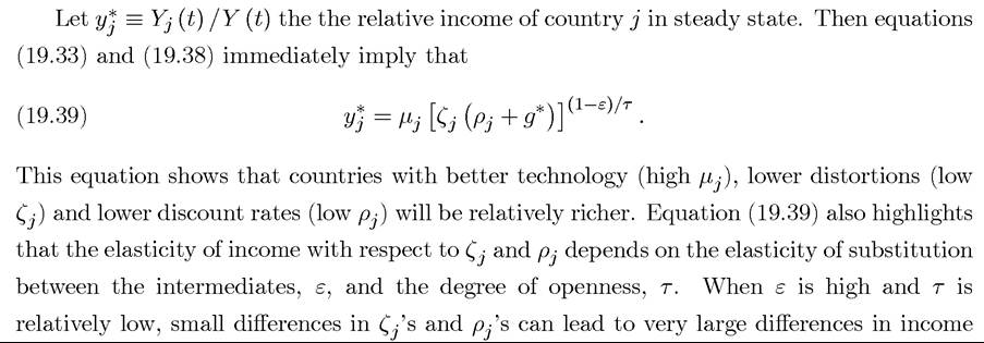
across countries. This observation is interesting for another reason; recall from Chapters 2 and 3 that the Solow growth model generates a similar equation linking the world income 779

distribution to differences in savings rates and technology. In particular, recall that in a world with a Cobb-Douglas aggregate production function and no human capital differences, the Solow model implies that (19.40) where Aj is the relative labor-augmenting productivity of country j, Sj is its savings rate, g* is again the world growth rate and α is the exponent of capital in the Cobb-Douglas production function, which is also equal to the share of capital in national income. Equation (19.39) shows that the implications of the world economy with trade are very similar, except that

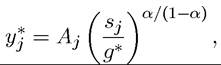
(1) the role of the labor-augmenting technologies is played by the technological capabilities of the country, which determine the range of goods in which it has a comparative advantage;

(2) the role of the saving rate is played by the discount rate ρj and the policy parameter affecting the distortions on the production of investment goods, ζj; (3) instead of the share of capital in national income, the elasticity of substitution between intermediates and the degree of trade openness affects how spread out the world income distribution is. Exercise 19.15 develops these points further.

19.4.3. The General Model*. The model presented in the previous subsection has a number of striking implications. The most important is that despite the possibility of endogenous growth at the country level, world relative prices adjust in such a way as to keep the world income distribution stable. Consequently, differences in preferences and technology across countries translate into differences in income levels along a stable income distribution, rather than into differences in permanent growth rates. However, the reader may wonder how general this result is. The result was derived in the context of a collection of AK economies. In this subsection, I will show that the results generalize to an economy in which both capital and labor are used. To maintain the tractability of the model of the previous subsection, and in fact in order to obtain almost identical equations to those from the previous subsection, I will make use of the structure of production first used by Rebelo (1991), which we encountered in Section 11.3 in Chapter 11, where the production of investment goods only uses capital, while the production of consumption goods uses both capital and labor. While the exact mathematical derivations here depend on these specific assumptions, the general insights do not.

More specifically, preferences, demographics, the production functions for intermediates and the production function for investment goods are as same as in the previous subsection. The main difference is that the production function for consumption goods has now changed to

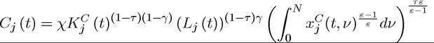
for some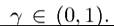Here χ is again a normalizing constant and where Lj (t) is the total

labor supply of country j at time t. All of this labor supply is used in the production of the consumption good, since neither the production of intermediates nor the production of the investment good use labor. The labor endowment in the economy is supplied inelastically by the representative household in the economy, and without loss of any generality, we normalize Lj (t) = 1. This implies that in terms of (19.20), Wj (t) stands both for the wage rate per unit of labor and total labor income. The associated unit cost function for the consumption good is

Using the same price normalization, i.e., (19.31), we continue to have (19.22) for intermediate prices and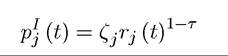

for the price of the investment good. The price of the consumption good is obtained, with a similar reasoning, as

The maximization problem of the representative household in each country is essentially unchanged, except for the stream of labor income that the individual will receive. This maximization problem again leads to the necessary and sufficient conditions given by (19.28) and (19.29). Combining these two equations, we again obtain that consumption expenditure is given as the fraction of the lifetime wealth of the individual, which now consists of the value of capital plus the discounted value of future labor earnings (see Exercise 19.16):

It is also straightforward to show that (19.33) still gives the necessary trade balance equation for each country.

The final condition we need to impose is market clearing for labor. Recall that labor demand comes only from the consumption goods sector, and given the Cobb-Douglas as­sumption, this demand is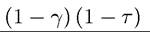times consumption expenditure,divided by

the wage rate, W_j. So the market clearing condition for labor in country j at time t is:

(19.43)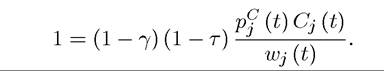

Finally, because (19.43) implies labor income, Wj (t), is always proportional to consump­tion expenditure, the optimal consumption rule, (19.42), can be simplified to the following 781

convenient equation:

In other words, households again consume a constant fraction of the value of the capital stock, but this fraction now depends not only on their discount rate, ρj, but also on the technology parameters, τ and γ. In light of this derivation, the following two propositions are straightforward:

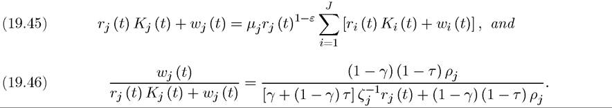
Proposition 19.11. In the general model with labor, the world equilibrium is character­ized by (19.34) for each j and t, as well as two additional equations

Proof. See Exercise 19.17. ?

The derivation and the intuition for this result follow the equilibrium characterization in the previous subsection. For a given cross section of capital stocks, equations (19.45) and (19.46) determine the cross section of rental rates and wage rates, and given the cross­sectional rental rates, (19.34) determines the evolution of the distribution of capital stocks in the world economy.

The next proposition shows that the structure of the world equilibrium is essentially identical to that in the previous subsection.

PROPOSITION 19.12. There exists a unique steady-state world equilibrium. In this equi­librium, capital stock and output in each country grows at the constant rate g* as in (19.36) above, and the world steady-state growth rate g* is the unique solution to (19.37). This unique steady-state equilibrium is global ly stable.

Proof. See Exercise 19.18. ?

This proposition implies that the results regarding the stable income distribution continue to apply in this more general model. Moreover, equation (19.39) still gives the world income distribution in the steady-state world equilibrium.

The more general model does not simply replicate the results on the simpler AK model, however. One important implication of this more general model concerns the relative prices of investment and consumption goods. As discussed previously, the empirical evidence strongly suggests that the price of investments goods relative to consumption goods is greater in poor countries. Many models adopt a reduced-form approach to this empirical regularity and 782

argue that it must be due to frictions affecting the investment sector in poor economies. However, only models that allow for trade and different production function for consumption and investment goods can be truly useful for understanding the sources of differences in these relative prices. The current model, which incorporates these features, naturally generates this pattern of relative prices. The equilibrium derivation above immediately implies the following relative price in each country:

so that the relative price of investment goods will be higher in countries that have high ζj and low wages. The first part of this result, that countries with high ζj's (high distortions on investment good sectors) have higher relative prices of investment goods, is consistent with the presumption in the literature. However, equation (19.46) above shows that countries with worse technology (low μj) and higher discount rates (high ρj) will also have lower wages and, via this channel, they will have higher relative prices of investment goods. Therefore, the current model not only provides us with a tractable framework for the analysis of interna­tional trade of economic growth, and how trade acts as a force stabilizing the world income distribution, but it also generates a cross section of the relative prices of investment and consumption goods that is consistent with the patterns we observe in the data. Furthermore, it highlights that the relative price of investment goods may vary across countries for reasons different from distortions on the investment sector, so that considerable care is necessary when using the observed variation in these relative prices in context of one-sector and/or closed-economy models as the previous literature has done.

In concluding this section, let us return to a comparison of the economic forces emphasized here with those of Section 19.3. Recall that in the model of the previous section, each country takes the world product and factor prices as given, and then accumulates without running into diminishing returns to scale. In contrast, the model in this section has emphasized how capital accumulation by a country will increase the world supply of goods in which it specializes, thus creating powerful terms of trade effects. These terms of trade effects are the reason why the long-run world income distribution is stable and the fast-growing countries tend to increase the growth rate of the rest of the world. Can the approaches in these two sections be reconciled? I believe the answer is yes. One way to reconcile these two approaches is to view them as applying at different stages of development and for different kinds of goods. Imagine, for example, a world in which some goods are “standardized” and can be produced in any country. When a country is producing these goods, it does not face terms of trade effects and can accumulate without running into diminishing returns to capital. As discussed in the previous section, this might be a good approximation to the situation experienced by the East Asian tigers in the 1970s and 80s, when they specialized in medium-tech goods 783

(e.g., Vogel, 2006). However, as countries become richer they also produce and consume more specialized goods. These goods often come in differentiated varieties and thus a greater supply of any one of these goods will create terms of trade effects. Consequently, if a country is in the stage of development where it produces more of the specialized goods, further capital accumulation will run into diminishing returns because of terms of trade effects. An interesting research area is to construct models combining these two forces and determining when one becomes more important than the other. Whether a model that combines these forces will also generate new results (thus being more than the sum of its parts) is also an open question.

19.5.