Economic Growth in a Heckscher-Ohlin World
We have so far focused on the growth implications of trade in financial assets, which enables countries to change the time profile of their consumption. Perhaps more important is international trade in commodities, which allows countries to exploit their comparative advantages (resulting from technology or differences in factor proportions).
We now turn to a simple model of growth in a world consisting of countries that trade in commodities. This model builds on work by Ventura (1997), who constructed a tractable model of world equilibrium based on the Heckscher-Ohlin model of trade.The Heckscher-Ohlin model is the benchmark model of international trade. It posits that countries have access to the same (or similar) technologies, and the main source of trade is differences in factor proportions—that some countries have more capital relative to labor than others or more human capital than others, etc. Clearly, an analysis of such an economy necessitates the specification of models in which there are multiple commodities used either in consumption or used as intermediates in the production of a final good. For the sake of concreteness, we will pursue the second alternative as in the models in Chapter 15, though this is without any loss of generality.
In particular, we assume that each country has access to an aggregate production function of the following form:

where Yj (t) is final output in country j at time t, F denotes a constant returns to scale production function, with the usual characteristics (in particular, satisfying Assumptions 1 and 2), except that it is defined over two intermediate inputs rather than labor and capital. Notice that Assumption 2 also incorporates the Inada conditions, which will play an important 760
role in the analysis below.
These intermediate inputs, Xj (t) and XjK (t) are respectively labor and capital intensive. We use the letter X to denote these inputs, since they refer to the amounts of these inputs used in production rather than the amount of inputs produced in country j. In the presence of international trade these two quantities will typically differ. We assume throughout that the production of the final good is competitive.The theory of international trade is a well-developed and rich area of economics, and provides useful and fairly general theorems about the structure of production and trade. Here our purpose is not to review these results, but to illustrate the implications of Heckscher- Ohlin type international trade for economic growth, thus we assume the simplest possible setting in which the two intermediate inputs are each produced by one factor. In particular, we assume
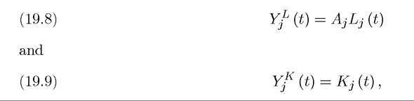
where the use of Y instead of X here emphasizes that these quantities refer to the local production, not the use, of these intermediates. Also, as usual, Lj (t) is total labor input in country j at time t, supplied inelastically, and Kj (t) is the total capital stock of the country. One feature about these intermediate production functions is worth noting: we have allowed productivity differences across countries in the production of the labor-intensive good, but not in the production of the capital-intensive good. This is the same assumption as the one adopted in Ventura (1997). Exercise 19.9 shows the implications of allowing differences in the productivity of the capital-intensive sector as well. For now, it suffices to note that this assumption makes it possible to derive a well-behaved world equilibrium, and is in the spirit of allowing only labor-augmenting technological progress in the basic neoclassical model. Moreover, this assumption is not entirely unreasonable, since we may think of differences in Aj's as reflecting differences in the human capital embodied in labor.
Notice also that we have not introduced any technological progress. This is again to simplify the exposition, and Exercise 19.10 extends the model in this section to incorporate laboraugmenting technological progress.Throughout the rest of this chapter, we assume that there is free international trade in commodities—in intermediate goods. This is an extreme assumption, since trading internationally involves costs, and many analyses of international trade incorporate the physical costs of transportation and tariffs. The main insights for economic growth do not depend on whether or not there are such costs, so I will simplify the analysis by assuming costless international trade. The most important implication of this assumption is that the prices of traded commodities, here the intermediate goods, are the same in all countries and are 761
equal to their “world prices”. Then the world supply and demand for these commodities will determine these prices. In particular, we denote the world price of the labor-intensive intermediate at time t by pL (t) and the price of the capital-intensive intermediate by pκ (t). Both of these prices are in terms of the final good in the world market, which is taken as numeraire, with price normalized to 1.1
Given the production technologies in (19.8) and (19.9), this immediately implies that factor prices, the wage rate and the rental rate of capital in country j at time t are given by 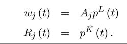 These two equations summarize the most important economic insights of the model studied here. Factor prices shape the incentives to accumulate capital in the neoclassical growth model and are typically determined by the capital-labor ratio (recall Chapter 8). The specific structure we have here, in contrast, implies that these factor prices are determined by world prices. In particular, since capital is used only in the production of the capital-intensive intermediate and there is free trade in intermediates, the rental rate of capital in each country is given by the world price of the capital-intensive intermediate.
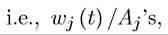 that are equalized. We follow Trefler (1993) in referring to this pattern as conditional factor price equalization across countries, meaning that, once we take into account intrinsic productivity differences of factors, there is equalization of factor prices across countries. Conditional factor price equalization is weaker than the celebrated factor price equalization of international trade theory, which would require Wj (t)'s to be equalized across countries. Instead we have that Wj (t) /Aj's are equalized.
 In this model, equalization of factor prices (or conditional factor prices) is an immediate consequence of free trade in goods, since each factor is only used in the production of a single traded intermediate. Nevertheless, factor price equalization results are considerably more general than the specialized structure here might suggest. In particular, factor price equalization or conditional factor price equalization results apply in general international trade models without trading frictions under fairly weak assumptions. Intuitively, trading commodities is a way of trading factors; if there is sufficient trade in commodities—especially sufficient trade in commodities with different factor intensities—then countries that are more
1In this model, there is no loss of generality in assuming that the price of the final good is normalized to 1 in each country even if there is no trade in final good. This is because all goods are traded and there are no differences in costs of living (purchasing power parity) across countries. This will no longer be the case in the model we study in the next section. Throughout, we take no position on whether there is trade in the final good, but, as specified below, we do not allow international lending and borrowing.
abundant in one factor will sell enough of the goods embedding that factor to equalize factor prices across countries.
In the jargon of international trade theory, with free trade of commodities, there will exist a cone of diversification, such that when factor proportions of different countries are within this cone, there will be (conditional) factor price equalization. Our extreme assumption that labor is used in the production of the labor-intensive intermediate and capital is used in the production of the capital-intensive intermediate is useful as it ensures that the cone of diversification is large enough to include any possible configuration of the distribution of capital and labor stocks across countries.The reader may also wonder why conditional factor price equalization is important. Its main importance for us is that when there is conditional factor price equalization, factor prices in each country are entirely independent of its capital stock and labor (provided that the country in question is “small” relative to the rest of the world; recall footnote 1 in the previous chapter). Thus each country will be taking intermediate prices, and consequently factor prices, as given when it makes its allocation and accumulation decisions. In fact, the distinguishing feature of the model analyzed in this section is this independence of factor prices from accumulation decisions, which is, in turn, a direct implication of a world of Heckscher-Ohlin trade.
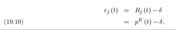
We also assume that as in previous chapters, capital depreciates at an exponential rate δ in each country, so that the interest rate is
We next specify the resource constraints facing the economy. While there is free international trade in commodities, we assume that there is no international trade in assets. Thus we will be abstracting from the issues of international lending and borrowing discussed in the previous two sections. This will enable us to isolate the effects of international trade in the simplest possible way.
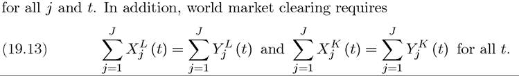
Lack of international lending and borrowing implies that at every date, each country must run a balanced international trade. In terms of the variables introduced so far, this implies the following trade balance equation:
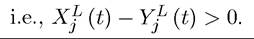
for all j and all t. This equation is intuitive; it requires that for each country (at each date) the value of their net sales of the capital-intensive good should be made up by their net purchases of the labor-intensive good. For example, if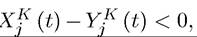 so that the country is a net
supplier of the capital-intensive good (i.e., it uses less of the capital-intensive good in its final good sector than it produces), then it must be a net purchaser of the labor-intensive good,
763
In addition to this trade balance equation, there is the usual resource constraint affecting each country at each time, which we can write as

The important feature in this equation is that both the consumption good and the capital good are produced with the same technology—one unit of the final good can be transformed into one unit of consumption good or one unit of capital or the investment good. In the next section, we will see how different factor intensities of consumption and capital goods can be allowed in models of international trade and growth. But for now, the simpler setup with the consumption and investment goods having the same factor intensities is sufficient for our purposes.
Finally, on the preference side, we assume that each country admits a representative household with standard preferences

where is per capita consumption in country j at time t and we have
imposed that all countries have the same time discount rate, ρ, and also the same rate of population growth. Throughout this section, without loss of any generality, we assume that all the decisions within each country is made by the representative household of that country, and we assume that p > n to ensure positive discounting and finite lifetime utilities (see Chapter 8, in particular, Assumption 40).
With a reasoning similar to that in Chapter 8, a key object is the ratio of “capital-like” intermediates relative to “labor-like” intermediates in production. For this reason, we define
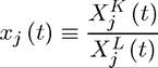
so that
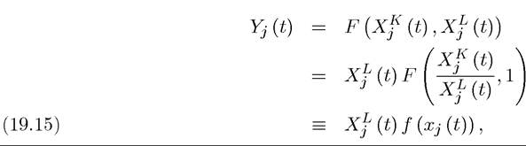
where the third line de fines the function f (∙) in the usual way exploiting the constant returns to scale nature of the function F. We refer to Xj (t) as the capital intermediate intensity of
country j. We also define kj (t) ? Kj (t) /Lj (t) as the capital labor ratio in country j at time t.
A world equilibrium can be expressed as a sequence of consumption, capital accumulation and capital intermediate intensity decision for each country and world prices, i.e.,  maximizes the utility of the representative household in country j subject to (19.11) and (19.12) given the sequence the world prices
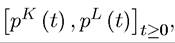 and world prices are such that world markets
clear, i.e., the equations in (19.13) hold. A steady-state world equilibrium is defined similarly as an equilibrium in which all of these quantities are constant.
Let us start with a straightforward result about the allocation of production around the world:
Proposition 19.5. Consider the above-described model. In any world equilibrium we
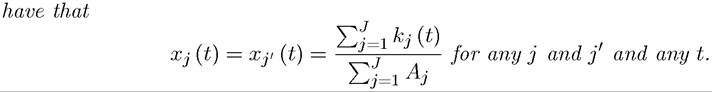
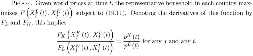
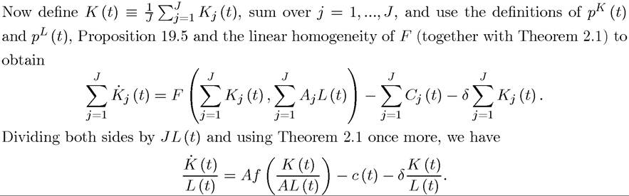
Using the definition in (19.15) and the linear homogeneity of F, this can be written as
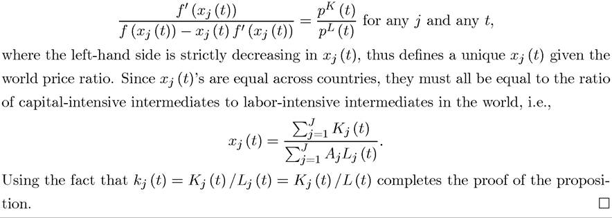
This proposition implies that irrespective of differences and capital-labor ratios across countries, the ratio of capital-intensive to labor-intensive intermediates in production will be equalized across countries.
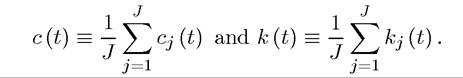
The equalization of the use of the ratio of capital-intensive to labor-intensive intermediates in the production of the final good enables us to aggregate the production and capital stocks 765
of different countries to obtain the behavior of world aggregates. In particular, let c (t) be the average consumption per capita in the world and k (t) be the average capital-labor ratio in the world, given by
The next proposition shows that world aggregates follow laws of motion very similar to that of the standard neoclassical closed economy.
PROPOSITION 19.6. Consider the above-described model. Then in any world equilibrium, the world averages follow the laws of motion given by

where r (t) = pκ (t) is the world interest rate at time t and
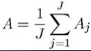
is average labor productivity.
Proof. Using (19.11), (19.12) and Proposition 19.5, the law of motion of the capital stock of country j can be written as

Using the definition of k (t) gives the second differential equation.
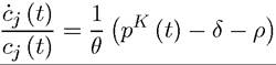
To obtain the differential equation for c(t), aggregate the Euler equation for the representative household in each county, for each j. This completes
the proof of the proposition. ?
The result in this proposition is not surprising. With (conditional) factor price equalization, the world behaves as an integrated closed economy, and thus obeys the two key 766
differential equations of the neoclassical model. Now using the previous two propositions, we can characterize the form of the steady-state world equilibrium.
PROPOSITION 19.7. Consider the above-described model. There exists a unique steadystate equilibrium whereby
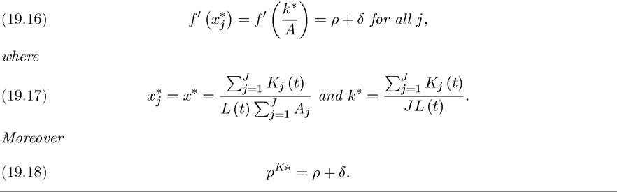
Proof. The proof follows from Proposition 19.6. The Inada conditions in Assumption 2 rule out sustained growth. Therefore, world average consumption must remain constant in steady state, and the interest rate must satisfy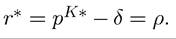 Propositions 19.5 and 19.6
then yield (19.16) and (19.17). ?
Proposition 19.7 shows that the steady-state world equilibrium takes a very simple form, with the ratio of capital-intensive to labor-intensive intermediates pinned down purely by the aggregate production function F (or its transform, f) and by the ratio of total capital to total labor in the world. The reason why steady-state production structure is determined by world supplies of capital and labor is simple: in the presence of (conditional) factor price equalization, the world economy is effectively integrated. We have already seen in the previous two sections how capital flows can make the world become integrated. The analysis in this section shows that Heckscher-Ohlin trade also leads to the same result (as long as it guarantees conditional factor price equalization).
While the structure of the steady-state equilibrium is rather straightforward, transitional dynamics in this world economy are somewhat more involved. In fact, the behavior of individual economies can be quite rich and complicated. Nevertheless, the fact that world averages obey the equations of the neoclassical growth model ensures that the steady-state world equilibrium is globally stable.
PROPOSITION 19.8. Consider the above-described economy. The steady-state equilibrium characterized in Proposition 19.7 is globally saddle-path stable.
Proof. With the arguments in the proof of Proposition 19.6, we have that for any sequence of world prices the problem of the representative household in
each country j at any time t satisfies the differential equations:

Standard arguments from Chapter 8 applied to world averages in Proposition 19.6 imply that world averages converge to the unique world steady state equilibrium and converges to ρ + δ. This immediately implies that the law of motion for the consumption and capital-labor ratio of each country also converges. With
 the convergence is
necessarily to the unique steady-state world equilibrium. ?
The analysis so far showed that a world economy consisting of a collection of economies engaged in Heckscher-Ohlin trade generates a pattern of growth similar to that we have seen in Chapter 8, with each country converging to a unique steady state. There is one important difference, however. As in the model with international borrowing and lending in the previous section, the nature of the transitional dynamics is very different from the closed-economy neoclassical growth models. Here, despite the absence of international capital flows, the rate of return to capital is equalized across countries. Thus there are no transitional dynamics resulting from a country with a higher rate of return to capital accumulating capital faster than the rest. This model therefore also emphasizes the potential pitfalls of using the closed- economy growth model for the analysis of output and capital dynamics across countries and regions.
Nevertheless, the results on transitional dynamics are perhaps the less interesting implications of the current model. One of my main objectives in this chapter is to illustrate how the presence of international trade changes the conclusions of closed economy growth models. The current framework already points out how this can happen. Notice that while the world economy has a standard neoclassical technology satisfying Assumptions 1 and 2, each country faces an “AK” technology, since it can accumulate as much capital as it wishes without running into diminishing returns. In particular, for every additional unit of capital at time t, a country receives a return of pκ (t), which is independent of its own capital stock. So how is it that the world does not generate endogenous growth? The answer is that while each country faces an AK technology, and thus can accumulate when the price of capital-intensive intermediates is high, accumulation by all countries drives down the price of capital-intensive intermediate goods to a level that is consistent with steady state. In other words, the price of capital-intensive intermediates will adjust to ensure the steady state equilibrium where capital, output and consumption per capita are constant (see the proof of Proposition 19.8). While this process describes the long-run dynamics, it also opens the door for a very different 768
type of short run (or “medium run”) dynamics, especially for countries that have different saving rates than others.
To illustrate this possibility in the simplest possible way, consider the following thought experiment. Let us start with the world economy in steady state and suppose that one of the countries experiences a decline in its discount rate from ρ to ρ' < p. What will happen? The answer is provided in the next proposition.
PROPOSITION 19.9. Consider the above-described model. Suppose J is arbitrarily large and the world starts in steady state at time t = 0, then the discount rate of country 1 declines to ρ' < p. After this change, there exists some T > 0 such that for all t ∈ [0,T), country one

Proof. In steady state, Proposition 19.8 and equation (19.18) imply that
Since country 1 faces this price as the return on capital and has a lower discount factor ρ', we are in the AK world of Chapter 11, Section 11.1, and the cost and growth rate follows from the analysis there. ?
Essentially, given conditional factor-price equalization, each country faces an AK technology, thus can accumulate capital and grow without running into diminishing returns. The price of capital-intensive intermediates and thus the rate of return to capital is pinned down by the discount rate of other countries in the world, so that country 1, with its lower discount rate, will have an incentive to save faster than the rest of the world and can achieve positive growth of income per capita (while the rest of the world has constant income per capita).
Therefore, the model of economic growth with Heckscher-Ohlin trade can easily rationalize bouts of rapid growth (“growth miracles”) by the countries that change their policies or their savings rates (or discount rates). Ventura (1997) suggests this model is a potential explanation for why, starting in the 1970s, East Asian tigers may have grown rapidly without running into diminishing returns. Since in the 1970s and 1980s East Asian economies were indeed more open to international trade than many other developing economies and have accumulated capital rapidly (e.g., Young, 1992, 1995, Vogel, 2006), this explanation is quite plausible. It shows how international trade can temporarily prevent the diminishing returns to capital that would set in because of rapid accumulation and enable sustained growth at higher rates.
Nevertheless, such behavior cannot go on forever. This follows from Assumption 2 above, which implies that world output cannot grow in the long run. So how is Proposition 19.9 consistent with this? The answer is that this proposition describes behavior in the “medium run”. This is the reason why the statement of the proposition is for t ∈ [0,T). At some 769
point, country 1 will become so large relative to the rest of the world that it will essentially own almost all of the capital of the world. At that point or in fact even before this point is reached, country 1 can no longer be considered a “small” country; it will have a major impact, and it will recognize this impact, on the relative price of the capital-intensive intermediate. Consequently, the rate of return on capital will eventually fall so that accumulation by this country comes to an end. Naturally, an alternative path of adjustment could take place if, at some future date, the discount rate of country 1 increases back to ρ, so that the world economy again settles into a steady state.
The important lesson from this discussion is that while the current model can generate growth miracles, these can only apply in the “medium run”. The fact that growth miracles can happen only in the medium run highlights another important feature of the current model. Exercise 19.8 shows that the current model does not admit a steady-state equilibrium (or even a well defined distribution of world income) when discount rates differ across countries. In other words, the well behaved world equilibrium in the world income distribution that emerges from this model relies on the knife-edge case in which all countries have the same discount rate (and also the same productivity of the capital-intensive intermediates, see Exercise 19.9). This feature is not only a shortcoming of the current model, but more generally a shortcoming of all Heckscher-Ohlin approach to trade and growth. In the traditional Heckscher-Ohlin model there is no comparative advantage coming from technology, so that each country is either small and takes world prices as given, or becomes sufficiently large to influence world prices for all commodities. This seems an unappealing feature on both empirical and intuitive grounds; while it is plausible that countries take prices of the goods that they import as given, they often influence the world prices of at least some of the goods that they export (such as copper for Chile, Microsoft windows for the United States or Lamborghinis for Italy). In the next section, we will see that models with more Ricardian features avoid these unappealing implications and provide a richer and more tractable framework for the analysis of the interaction between international trade and economic growth.
19.3.