The Economic Environment of the Basic Solow Model

Economic growth and development are dynamic processes, focusing on how and why output, capital, consumption and population change over time. The study of economic growth and development therefore necessitates dynamic models.

The Solow model can be formulated either in discrete or in continuous time. We start with the discrete time version, both because it is conceptually simpler and it is more com­monly used in macroeconomic applications. However, many growth models are formulated in continuous time and we will also provide a detailed exposition of the continuous-time version of the Solow model and show that it is often more tractable.

2.1.1. Households and Production. Consider a closed economy, with a unique final good. The economy is in discrete time running to an infinite horizon, so that time is indexed by t = 0,1, 2,.... Time periods here can correspond to days, weeks, or years. So far we do not need to take a position on this.

The economy is inhabited by a large number of households, and for now we are going to make relatively few assumptions on households because in this baseline model, they will not be optimizing. This is the main difference between the Solow model and the neoclassical growth model. The latter is the Solow model plus dynamic consumer (household) optimization. To fix ideas, you may want to assume that all households are identical, so that the economy admits a representative household—meaning that the demand and labor supply side of the 32

economy can be represented as if it resulted from the behavior of a single household. We will return to what the representative household assumption entails in Chapter 5 and see that it is not totally innocuous.

What do we need to know about households in this economy? The answer is: not much. We do not yet endow households with preferences (utility functions). Instead, for now, we simply assume that they save a constant exogenous fraction s of their disposable income— irrespective of what else is happening in the economy. This is the same assumption used in basic Keynesian models and in the Harrod-Domar model mentioned above. It is also at odds with reality. Individuals do not save a constant fraction of their incomes; for example, if they did, then the announcement by the government that there will be a large tax increase next year should have no effect on their saving decisions, which seems both unreasonable and empirically incorrect. Nevertheless, the exogenous constant saving rate is a convenient starting point and we will spend a lot of time in the rest of the book analyzing how consumers behave and make intertemporal choices.

The other key agents in the economy are firms. Firms, like consumers, are highly het­erogeneous in practice. Even within a narrowly-defined sector of an economy (such as sports shoes manufacturing), no two firms are identical. But again for simplicity, we start with an assumption similar to the representative household assumption, but now applied to firms. We assume that all firms in this economy have access to the same production function for the final good, or in other words, we assume that the economy admits a representative firm, with a representative (or aggregate) production function. Moreover, we also assume that this aggregate production function exhibits constant returns to scale (see below for a definition). More explicitly, the aggregate production function for the unique final good is

(2.1) Y (t) = F [K (t),L (t),A (t)]

where Y (t) is the total amount of production of the final good at time t, K (t) is the capital stock, L (t) is total employment, and A (t) is technology at time t. Employment can be measured in different ways.

consumption and as an input, as “seed”, for the production of more corn tomorrow. Capital then corresponds to the amount of corn used as seeds for further production.

Technology, on the other hand, has no natural unit. This means that A (t), for us, is a shifter of the production function (2.1). For mathematical convenience, we will often represent A (t) in terms of a number, but it is useful to bear in mind that, at the end of the day, it is a representation of a more abstract concept. Later we will discuss models in which A (t) can be multidimensional, so that we can analyze economies with different types of technologies. As noted in Chapter 1, we may often want to think of a broad notion of technology, incorporating the effects of the organization of production and of markets on the efficiency with which the factors of production are utilized. In the current model, A (t) represents all these effects.

A major assumption of the Solow growth model (and of the neoclassical growth model we will study in Chapter 8) is that technology is free; it is publicly available as a non-excludable, non-rival good. Recall that a good is non-rival if its consumption or use by others does not preclude my consumption or use.

As an aside, you might want to note that some authors use x_t or K_t when working with discrete time and reserve the notation x (t) or K (t) for continuous time. Since we will go back and forth between continuous time and discrete time, we use the latter notation throughout. When there is no risk of confusion, we will drop time arguments, but whenever there is the slightest risk of confusion, we will err on the side of caution and include the time arguments.

Now we impose some standard assumptions on the production function.

Assumption 1. (Continuity, Differentiability, Positive and Diminishing Mar­ginal Products, and Constant Returns to Scale) The production function F : is twice continuously differentiable in K and L, and satisfies

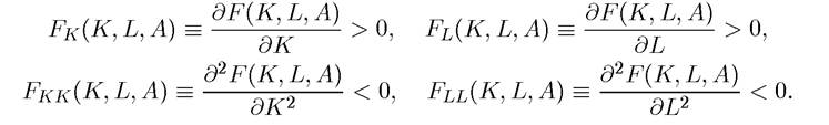
Moreover, F exhibits constant returns to scale in K and L.

All of the components of Assumption 1 are important. First, the notation F : R∣ → R∣∣ implies that the production function takes nonnegative arguments (i.e., K, L ∈ R∣) and maps to nonnegative levels of output (Y ∈ R∣). It is natural that the level of capital and the level of employment should be positive. Since A has no natural units, it could have been negative. But there is no loss of generality in restricting it to be positive. The second important aspect of Assumption 1 is that F is a continuous function in its arguments and is also differentiable. There are many interesting production functions which are not differentiable and some interesting ones that are not even continuous. But working with continuously differentiable functions makes it possible for us to use differential calculus, and the loss of some generality is a small price to pay for this convenience. Assumption 1 also specifies that marginal products are positive (so that the level of production increases with the amount of inputs); this also rules out some potential production functions and can be relaxed without much complication (see Exercise 2.6). More importantly, Assumption 1 imposes that the marginal product of both capital and labor are diminishing, i.e., Fkk < 0 and Fll < 0, so that more capital, holding everything else constant, increases output by less and less, and the same applies to labor. This property is sometimes also referred to as “diminishing returns” to capital and labor. We will see below that the degree of diminishing returns to capital will play a very important role in many of the results of the basic growth model. In fact, these features distinguish the Solow growth model from its antecedent, the Harrod-Domar model (see Exercise 2.16).

The other important assumption is that of constant returns to scale. Recall that F exhibits constant returns to scale in K and L if it is linearly homogeneous (homogeneous of degree 1) in these two variables.

Definition 2.1. Let K be an integer. The function gis homogeneous of

degree m in x ∈ R and y ∈ R if and only if

It can be easily verified that linear homogeneity implies that the production function F is concave, though not strictly so (see Exercise 2.1).

Linearly homogeneous (constant returns to scale) production functions are particularly useful because of the following theorem:

Theorem 2.1. (Euler's Theorem) Suppose that g :is continuously differ­

entiable in x ∈ R and y ∈ R, with partial derivatives denoted by g_x and g_y and is homogeneous of degree m in x and y. Then

Moreover, g_x (x, y, z) and g_y (x, y, z) are themselves homogeneous of degree m — 1 in x and y.

Proof. We have that g is continuously differentiable and

Differentiate both sides of equation (2.2) with respect to λ, which gives

for any λ. Setting λ = 1 yields the first result. To obtain the second result, differentiate both sides of equation (2.2) with respect to x:

Dividing both sides by λ establishes the desired result. ?

2.1.2. Market Structure, Endowments and Market Clearing. For most of the book, we will assume that all factor markets are competitive. This is yet another assumption that is not totally innocuous. Both labor markets and capital markets have imperfections that have important implications for economic growth. But it is only by starting out with the competitive benchmark that we can best appreciate the implications of these imperfections for economic growth. Furthermore, until we come to models of endogenous technological change, we will assume that product markets are also competitive, so ours will be a prototypical competitive general equilibrium model.

As in standard competitive general equilibrium models, the next step is to specify en­dowments, that is, what the economy starts with in terms of labor and capital and who owns these endowments. Let us imagine that all factors of production are owned by households. In particular, households own all of the labor, which they supply inelastically. Inelastic sup­ply means that there is some endowment of labor in the economy, for example equal to the population, L(t), and all of this will be supplied regardless of the price (as long as it is nonnegative). The labor market clearing condition can then be expressed as:

(2.3) L (t) = L(t)

for all t, where L (t) denotes the demand for labor (and also the level of employment). More generally, this equation should be written in complementary slackness form. In particular, 36

let the wage rate (or the rental price of labor) at time t be w (t), then the labor market clearing condition takes the form L (t) ≤ L (t), w (t) ≥ 0 and (L (t) — L(t) w (t) = 0. The complementary slackness formulation makes sure that labor market clearing does not happen at a negative wage—or that if labor demand happens to be low enough, employment could be below L (t) at zero wage. However, this will not be an issue in most of the models studied in this book (in particular, Assumption 1 and competitive labor markets make sure that wages have to be strictly positive), thus we will use the simpler condition (2.3) throughout.

The households also own the capital stock of the economy and rent it to firms. We denote the rental price of capital at time t be R (t). The capital market clearing condition is similar to (2.3) and requires the demand for capital by firms to be equal to the supply of capital by households: K^s (t) = K^d (t), where K^s (t) is the supply of capital by households and K^d (t) is the demand by firms. Capital market clearing is straightforward to impose in the class of models analyzed in this book by imposing that the amount of capital K (t) used in production at time t is consistent with household behavior and firms’ optimization.

We take households’ initial holdings of capital, K (0), as given (as part of the description of the environment), and this will determine the initial condition of the dynamical system we will be analyzing. For now how this initial capital stock is distributed among the households is not important, since households optimization decisions are not modeled explicitly and the economy is simply assumed to save a fraction s of its income. When we turn to models with household optimization below, an important part of the description of the environment will be to specify the preferences and the budget constraints of households.

At this point, we could also introduce P (t) as the price of the final good at time t. But we do not need to do this, since we have a choice of a numeraire commodity in this economy, whose price will be normalized to 1. In particular, as we will discuss in greater detail in Chapter 5, Walras’ Law implies that we should choose the price of one of the commodities as numeraire. In fact, throughout we will do something stronger. We will normalize the price of the final good to 1 in all periods. Ordinarily, one cannot choose more than one numeraire— otherwise, one would be fixing the relative price between the two numeraires. But again as will be explained in Chapter 5, we can build on an insight by Kenneth Arrow (Arrow, 1964) that it is sufficient to price securities (assets) that transfer one unit of consumption from one date (or state of the world) to another. In the context of dynamic economies, this implies that we need to keep track of an interest rate across periods, denoted by r (t), and this will enable us to normalize the price of the final good to 1 in every period (and naturally, we will keep track of the wage rate w (t), which will determine the intertemporal price of labor relative to final goods at any date t).

This discussion should already alert you to a central fact: you should think of all of the models we discuss in this book as general equilibrium economies, where different commodi­ties correspond to the same good at different dates. Recall from basic general equilibrium theory that the same good at different dates (or in different states or localities) is a different commodity. Therefore, in almost all of the models that we will study in this book, there will be an infinite number of commodities, since time runs to infinity. This raises a number of special issues, which we will discuss as we go along.

Now returning to our treatment of the basic model, the next assumption is that capital depreciates, meaning that machines that are used in production lose some of their value because of wear and tear. In terms of our corn example above, some of the corn that is used as seeds is no longer available for consumption or for use as seeds in the following period. We assume that this depreciation takes an “exponential form,” which is mathematically very tractable. This means that capital depreciates (exponentially) at the rate δ, so that out of 1 unit of capital this period, only 1 — δ is left for next period. As noted above, depreciation here stands for the wear and tear of the machinery, but it can also represent the replacement of old machines by new machines in more realistic models (see Chapter 14). For now it is treated as a black box, and it is another one of the black boxes that will be opened later in the book.

The loss of part of the capital stock affects the interest rate (rate of return to savings) faced by the household. Given the assumption of exponential depreciation at the rate δ and the normalization of the price of the final goods to 1, this implies that the interest rate faced by the household will be r (t) = R (t) — δ. Recall that a unit of final good can be consumed now or used as capital and rented to firms. In the latter case, the household will receive R (t) units of good in the next period as the rental price, but will lose δ units of the capital, since δ fraction of capital depreciates over time. This implies that the individual has given up one unit of commodity dated t — 1 for r (t) units of commodity dated t. The relationship between r (t) and R (t) explains the similarity between the symbols for the interest rate and the rental rate of capital. The interest rate faced by households will play a central role when we model the dynamic optimization decisions of households. In the Solow model, this interest rate does not directly affect the allocation of resources.

2.1.3. Firm Optimization. We are now in a position to look at the optimization prob­lem of firms. Throughout the book we assume that the only ob jective of firms is to maximize profits. Since we have assumed the existence of an aggregate production function, we only need to consider the problem of a representative firm. Throughout, unless otherwise stated, we assume that capital markets are functioning, so firms can rent capital in spot markets. This implies that the maximization problem of the (representative) firm can be written as a 38

static program

When there are irreversible investments or costs of adjustments, as discussed in Section 7.8 in Chapter 7, we would need to consider the dynamic optimization problems of firms. But in the absence of these features, the production side can be represented as a static maximization problem.

A couple of additional feature are worth noting:

(1) The maximization problem is set up in terms of aggregate variables. This is without loss of any generality given the representative firm.

(2) There is nothing multiplying the F term, since the price of the final good has been normalized to 1. Thus the first term in (2.4) is the revenues of the representative firm (or the revenues of all of the firms in the economy).

(3) This way of writing the problem already imposes competitive factor markets, since the firm is taking as given the rental prices of labor and capital, w (t) and R (t) (which are in terms of the numeraire, the final good).

(4) This is a concave problem, since F is concave (see Exercise 2.1).

Since F is differentiable from Assumption 1, the first-order necessary conditions of the maximization problem (2.4) imply the important and well-known result that the competitive rental rates are equal to marginal products:

and

Note also that in (2.5) and (2.6), we used the symbols K (t) and L (t). These represent the amount of capital and labor used by firms. In fact, solving for K (t) and L (t), we can derive the capital and labor demands of firms in this economy at rental prices R (t) and w (t)—thus we could have used K^d (t) instead of K (t), but this additional notation is not necessary.

This is where Euler’s Theorem, Theorem 2.1, becomes useful. Combined with competitive factor markets, this theorem implies:

Proposition 2.1. Suppose Assumption 1 holds. Then in the equilibrium of the Solow growth model, firms make no profits, and in particular,

Proof. This follows immediately from Theorem 2.1 for the case of m = 1, i.e., constant returns to scale. ?

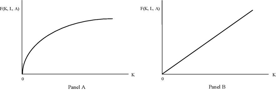
FIGURE 2.1. Production functions and the marginal product of capital. The example in Panel A satisfies the Inada conditions in Assumption 2, while the example in Panel B does not.

This result is both important and convenient; it implies that firms make no profits, so in contrast to the basic general equilibrium theory with strictly convex production sets, the ownership of firms does not need to be specified. All we need to know is that firms are profit-maximizing entities.

In addition to these standard assumptions on the production function, in macroeconomics and growth theory we often impose the following additional boundary conditions, referred to as Inada conditions.

Assumption 2. (Inada conditions) F satisfies the Inada conditions

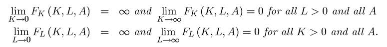
The role of these conditions—especially in ensuring the existence of interior equilibria— will become clear in a little. They imply that the “first units” of capital and labor are highly productive and that when capital or labor are sufficiently abundant, their marginal products are close to zero. Figure 2.1 draws the production function F (K,L,A) as a function of K, for given L and A, in two different cases; in Panel A, the Inada conditions are satisfied, while in Panel B, they are not.

We will refer to Assumptions 1 and 2 throughout much of the book.

2.2.