Transport costs and market size

The goal of this section is to study the effects on the growth process of partial seg­mentation in goods markets. The new model of globalization that I shall adopt here is as follows: at date t = 0 the costs of transporting some (but not all) goods across re­gions suddenly fall from prohibitive to negligible. In particular, I partition the set of all industries into the sets of tradable and nontradable industries, i.e. T_t and N_t such that T_t U N_t = I and T_t ∩ N_t = 0. The costs of transporting intermediate inputs and final goods fall from prohibitive to negligible at t = 0 if i ∈ T_t. But even after t = 0, the costs of transporting either the intermediate inputs, or the final goods, or both remain prohibitive if i ∈ N_t.⁶2 We keep assuming that the costs of transporting factors across regions remain prohibitive after t = 0, and that international trade in assets is not possi­ble.

A central aspect of the analysis turns out to be whether transport costs apply only to final goods, to intermediate inputs, or to both. Section 3.1 presents the case in which transport costs apply only to final goods. This model neatly generalizes the results ob­tained in the previous section. Section 3.2 studies the case in which transport costs apply only to intermediate inputs. This gives rise to agglomeration effects that can have a large and somewhat unexpected impact on the world income distribution. Section 3.3 analyzes the case in which transport costs apply to both final goods and intermediate in­puts. The interaction between the two types of frictions brings about a new perspective on the role of local markets.

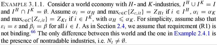
3.1. Nontraded goods and the cost of living

Consider next a world where some final goods are not tradable, although the interme­diate inputs required to produce them are always tradable. In particular, the costs of trading intermediate inputs are negligible for all i ∈ I, and the costs of transporting final goods are negligible if i ∈ T_t but prohibitive if i ∈ N_t. Since prices of final goods can differ across regions, a novel feature of this model is that regions will have different price levels.

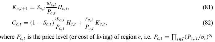
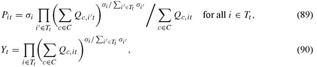
I must now revise the formal description of the model. While regional analogues of Equations (1) and (2) continue to apply, one must now recognize that final goods prices in nontradable industries might differ across regions. As a result, the price of consump­tion and investment will vary across them even if Equation (3) describing spending patterns still applies to all regions. Therefore, we must write the analogues of Equations (1) and (2) as follows:

for all c ∈ C.

Equation (83) replaces Equation (4). The latter obtains as the special case of the former in which all goods are tradable, i.e. T_t = I and N_t = 0. An implication of this choice of numeraire is that the price level of region c is equal to the ideal price index of its nontradable industries,

Since now price levels differ across regions it is necessary to distinguish between two concepts of income and factor prices: (1) market-based incomes and factor prices, i.e. Y_c,_t, w_ct and r_ct, and (2) real or PPP-adjusted incomes and factor prices, i.e. Y_ctt/P_c,_t, w_ctt∕P_ctt and r_ct/P_ct. Wheneverthere is no risk of confusion, I shall refer to the former simply as income and factor prices, and to the latter as real income and real factor prices. As before, Equations (5) and (6) describing technology apply to all regions, with the corresponding factor prices and industry productivities.

After globalization, producers of intermediate inputs in all industries and produc­ers of final goods in tradable industries face a global market and Equations (7)-(10) describing pricing policies, input demands and the free-entry condition therefore ap­ply only to those regions where the lowest-cost producers are located. But even after globalization, producers of final goods in nontradable industries remain sheltered from foreign competition, and Equations (7) and (8) apply to all regions and not only to the lowest-cost ones. Thus, Equation (44) no longer applies to the producers of final goods in nontradable industries [Equation (43) still stands as a definition, though].

Market clearing conditions are also affected by the presence of transport costs. While Equations (45) and (46) describing market clearing in regional factor markets still ap­ply, Equation (11) describing market clearing in global markets for final goods applies only to tradable industries. In nontradable industries, Equation (11) must be replaced by analogue conditions imposing market clearing in each regional market,

This completes the formal description of the model. For any admissible set of capital stocks, i.e. K_c0 for all c ∈ C; sequences for the vectors of savings, human capital and industry productivities, i.e. S_ct, H_ct and A_cc, for all c ∈ C and for all i ∈ I, and a sequence for the set N_t (or T_t), an equilibrium of the world economy after globalization consists of a sequence of prices and quantities such that the equations listed above hold at all dates and states of nature. Although there might be multiple geographical patterns of production that are consistent with world equilibrium, the assumptions made ensure that prices and world aggregates are uniquely determined.

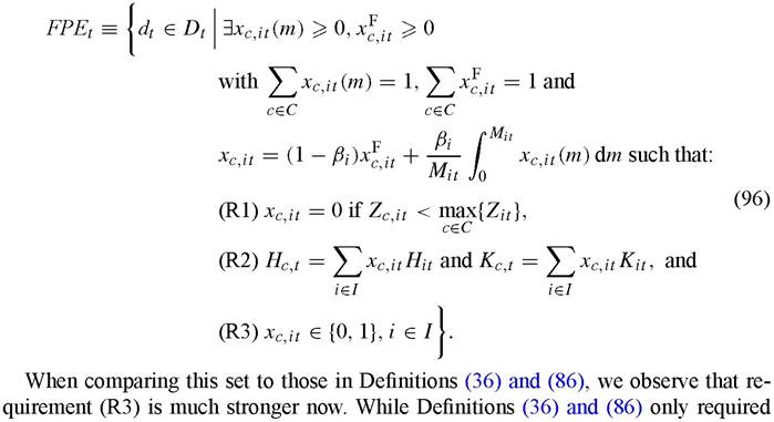
The best way to start the analysis is by asking again whether the assumed trade re­strictions matter at all. That is, to ask whether restricting factor mobility and now goods trade impede the world to achieve the level of efficiency of the integrated economy. Re-define the set FPE_t now as follows:

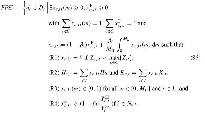
Comparing Definitions (36) and (86), we observe that the latter contains an additional requirement: each region should be able to produce all the final goods used for its own consumption and investment in nontradable industries. This additional restriction is a direct consequence of transport costs. The presence of this additional restriction reduces the size of FPE_t.

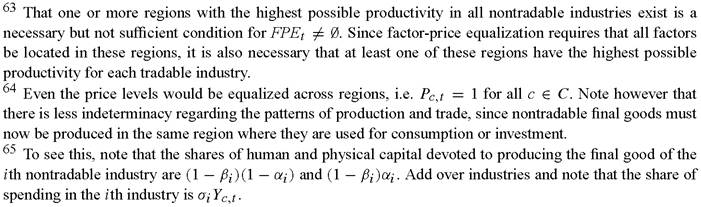
If d_t ∈ FPE_t, factor prices are equalized across regions and the world economy operates with the same efficiency as the integrated economy despite factor immobility and goods market segmentation. In this case, the world economy behaves exactly as the world of factor-price equalization of Section 2.2.⁶⁴ If d_t ∈ FPE_t, the world economy cannot operate at the same level efficiency as the integrated economy. As a result, either market-based factor prices, or real factor prices, or both differ across regions. But even in this case the behavior of the world economy does not depart much from what we observed in the worlds of Section 2. To see this, define H,^τ, and K^t_t as the factor endowments devoted to the production of tradable goods, i.e. all intermediate inputs and the final goods of tradable industries. Straightforward algebra shows that⁶⁵

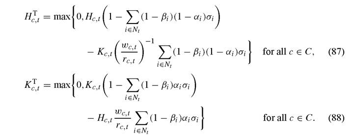
Equations (87) and (88) show the factor supplies that are left after subtracting from aggregate factor supplies the factors used in the production of final goods in nontradable industries. In the special case in which N_t = 0, these factor supplies equal the aggregate factor supplies and are independent of factor prices. But in the general case, these factor supplies depend on factor prices in the usual way. The higher is the wage-rental, the lower is the human to physical capital ratio used for the production of final goods in nontradable industries and, as a result, the higher is the relative supply of human to physical capital that is left after production of final goods in nontradable industries.

With Equations (87) and (88) at hand, it is straightforward to see that all the results in Sections 2.4 and 2.5 regarding incomes and factor prices still go through in the presence of nontradable final goods. Take, for instance, Example 2.4.1. Equations (47)-(48) must be rewritten as follows:

while Equations (49)-(52) still apply provided that we write Hj, and Kj_t instead of H_ci and K_ci, in Equations (49) and (50). Factor prices and the pattern of trade are determined by these modified versions of Equations (47)-(52) together with Equations (87) and (88). Since factor supplies are well behaved, a brief analysis of this system reveals that all the discussion of the properties of the world income distribution and its dynamics after Equations (58) and (59) still goes through. In fact, all the results and intuitions developed in the examples of Sections 2.4 and 2.5 still apply after we remove the assumption that N_t = 0.

The major difference between the world of this subsection and the one in Section 2 is that there is a discrepancy between market-based and real incomes and factor prices. To see this, we need to compute regional price levels. Equations (5)-(7) and (83) imply that

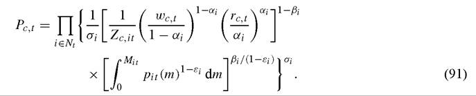
Since all regions face the same input prices, Equation (91) shows that, ceteris paribus, the price level is high in regions that have high factor prices and low productivity in non­tradable industries. This relationship is the first piece of a theory of the price level. The second piece is a relationship between factor prices, factor endowments and industry productivities. The following examples show how to obtain this additional relationship.

^[1] Note that this implies that all regions have the same productivity in nontradable industries. That is, Z_c i_t = Z_Ht if i ∈ N_t ∩ I^h and Z_cit = Z_κt if i ∈ N_t ∩ I^k for all c ∈ C.

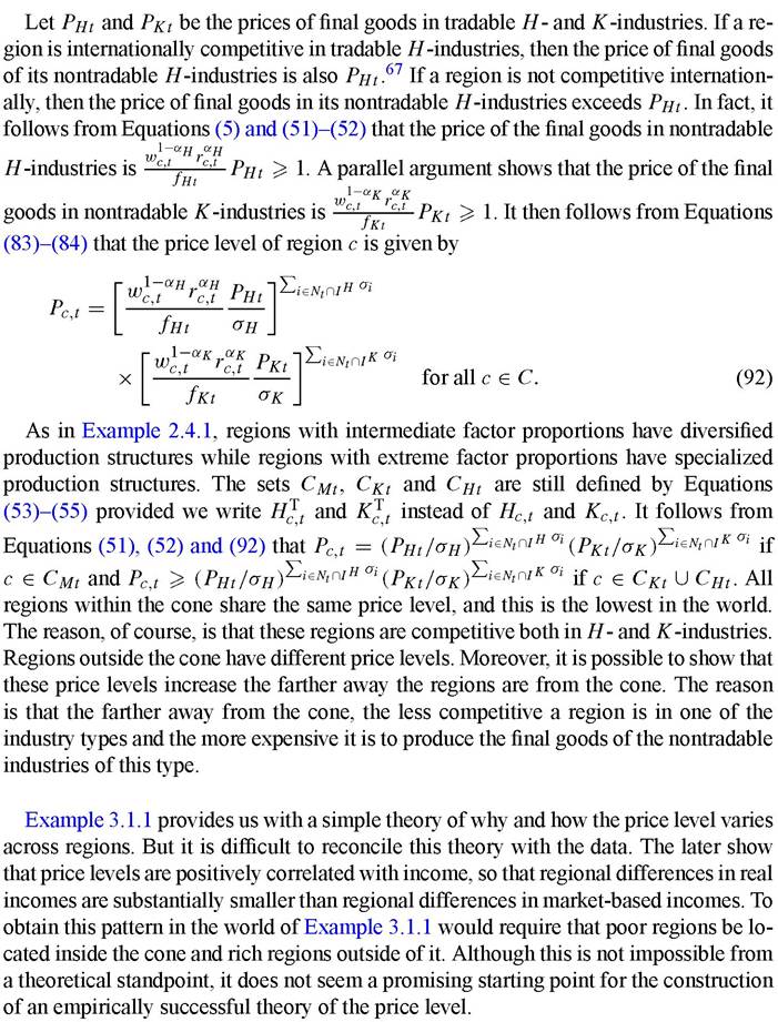
⁶⁷ This follows because the technology to produce final goods is the same for all H-industries, and also because the number of input varieties of H-industries does not depend on whether the industry is tradable or nontradable.

A positive association between incomes and price levels could arise somewhat more naturally in the world of Example 2.4.2 once we remove the assumption that N_t = 0. For instance, if nontradable industries tend to be more human-capital intensive than tradable industries the price level would be high in regions that belong to C_Kt, inter­mediate in regions that belong to C_Mt, and low in regions that belong to C_Ht. Assume then that most of the variation in income levels is due to differences in savings rates, so that rich regions are those that have low human to physical capital ratios. This does not seem implausible, since most nontradable industries tend to be in the service sector and this sector tends to use a higher human to physical capital ratio than other sec­tors.

More generally, in the worlds of Section 2.4 the correlation between income and price levels is positive or negative depending on how factor proportions vary with income and the factor intensities of nontradable industries relative to tradable ones. The central observation is that price levels should be high in regions that have factor proportions that are inadequate to produce nontradable goods. Building an empirically successful theory of the price level around this notion seems promising, although it remains to be done. Most of the existing research on the price level has focused instead on the role of regional differences in industry productivities. The next example presents a world where these differences generate a positive association between income and the price level.

industries.⁶⁸ Thisworldeconomy is akin to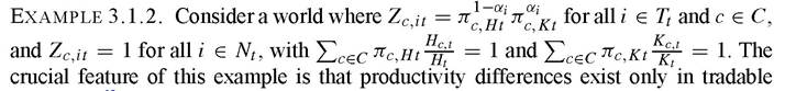that in Example 2.5.1. Forinstance, assume that there are H - and K -industries as in Examples 2.4.1 and 3.1.1. Then, we have that

industries are factor augmenting, regions with higher productivities have higher factor prices. Since there are no productivity differences in nontradable industries, regions with higher factor prices have a higher price level. Note that now a region inside the cone with high productivity in the tradable industries could have a higher price level than a region outside the cone with low productivity in the tradable industries.

⁶⁸ This assumption makes sense because nontradable industries consist mostly of services, and in the real world productivity differences in services seem small relative to productivity differences in agriculture or manufacturing.

In the world of this example, the price level is determined by a combination of two elements: how adequate are the region’s factor proportions to produce in the nontradable industries; and how high is the region’s productivity in the tradable industries relative to the nontradable ones. In the world of Example 3.1.1, this second force was not present and Equation (93) was reduced to Equation (92). We could also eliminate the first force by assuming that all regions belong to the cone, i.e. by assuming that there is conditional factor-price equalization. In this case, the price level is given by

In Equation (94) the only determinant of the price level is the level of productivity in the tradable industries. This special case is known as the Balassa-Samuelson hypothesis of why the price level is positively correlated with income. Higher productivity in the tradable industries is what makes regions both rich and expensive.

In addition to providing a theory of the price level, the world of this section is also useful because it allows us to study a smoother and more realistic version of the glob­alization process, i.e. a gradual reduction in the size of N_t. This is not only important for quantitative applications of the theory, but it also leads to new insights regarding the effects of globalization on welfare. The next example shows this.

Example 3.1.3. Consider a world economy with H - and K -industries, such that I^h U I^k = I and I^h ∩ I^k = 0. Assume α_i = 0 if i ∈ I^h and α_i = 1 if i ∈ I^k, and β_i = 0 for all i ∈ I. Within each type there are “advanced” and “backward” industries. A-regions have the highest possible productivity in all industries, regardless of whether they are “advanced” or “backward”. B-regions have the highest possible productivity only in “backward” industries. Up this point all the assumptions are as in Example 2.1.2, except that industry factor intensities are more extreme. Assume next that initially some industries are nontradable, i.e. N_t = 0, and consider a small step in the globalization process: some “advanced” H-industries become tradable, i.e. some elements of the set N_t ∩ I^h move into the set T_t ∩ I^h. What is the effect of this partial reduction in transport costs on regional incomes?

The reduction of transport costs leads to structural transformation: A-regions reduce their production in “backward” H-industries and increase their production in “ad­vanced” H-industries, while B-regions do the opposite.^[316] This increases efficiency and raises the combined world production of H -industries, lowering the price of their prod­ucts and therefore wages all over the world. Therefore, a partial reduction of transport costs has two effects: an increase in efficiency that lowers prices and benefits all regions, and a change in relative prices that benefits some regions but hurts others. A-regions with a large enough ratio of human to physical capital are worse off as a result of this partial reduction in transport costs.^[317] If coupled with an appropriate transfer scheme, partial globalization still constitutes a Pareto improvement for the world economy. But now this transfer scheme might require inter-regional transfers towards A-regions with large enough human to physical capital ratios.

The world of this subsection is a simple and yet very useful generalization of the world of Section 2. It allows us to study the sources of regional differences in price levels and also permits us to consider smoother versions of the globalization process. Despite this progress, the world of this subsection fails to capture a central aspect of transport costs because these only affect final goods. When transport costs affect intermediate inputs, they create incentives to agglomerate production in a single location. We study how this works next.

3.2. Agglomeration effects

Consider a world where transport costs apply only to intermediates, and not to final goods. In particular, assume that the costs of transporting inputs are negligible if i ∈ T_t but prohibitive if i ∈ N_t, while the costs of trading final goods are negligible for all i ∈ I.An implication of this last assumption is that the price level is the same in all regions and market-based and PPP-adjusted incomes coincide. But this does not mean that we are back to the worlds of Section 2. The inability of trading intermediate inputs creates an incentive to concentrate all the production of an industry in a single region. Only in this way, production of final goods can fully take advantage from the benefits of specialization. This force towards the agglomeration of economic activity has profound effects on the world income distribution and its dynamics.

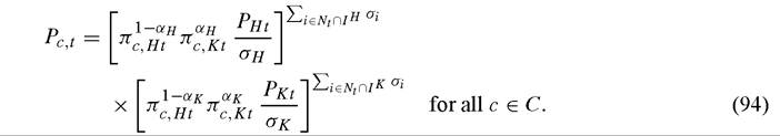
The formal description of the model is quite similar to that of Section 2.3. Regional analogues to Equations (1)-(3) apply. Since all regions share spending patterns and face the same final goods prices, the price of consumption and investment is the same for all, and we keep Equation (4) as the numeraire rule. Equations (5) and (6) describ­ing technology apply to all regions, with the corresponding factor prices and industry productivities. The only difference with the model of Section 2.2 is that, even after globalization, producers of intermediate inputs in nontradable industries remain shel­tered from foreign competition. As a result, in these industries Equations (9)-(10) apply to producers of intermediates in all regions and not only to the lowest-cost ones. Also Equation (8) applies to each region separately since only the demand from local produc­ers of final goods matters for the producers of intermediate inputs. Thus, Equation (44)

no longer applies to the producers of intermediate inputs in nontradable industries, and Equation (43) must be modified as follows:

Equation (95) simply recognizes that the number of intermediate inputs available and their prices can vary across regions.⁷¹ Finally, the market clearing conditions in Equa­tions (11), (45) and (46) apply.

This completes the formal description of the model. For any admissible set of capital stocks, i.e. K_c0 for all c ∈ C, and sequences for the vectors of savings, human capital and industry productivities, i.e. S_ct, H_ct and A_cit for all c ∈ C and for all i ∈ I, and a sequence for the set N_t (or T_t); an equilibrium of the world economy after globaliza­tion consists of a sequence of prices and quantities such that the equations listed above hold at all dates and states of nature. Like the other worlds we have studied up to this point, there might be multiple geographical patterns of production that are consistent with world equilibrium. Unlike the worlds we have studied up to this point however, there might also be multiple prices and world aggregates that are consistent with world equilibrium. This is, in fact, the most prominent feature of this world.

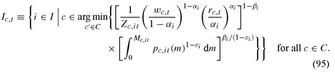
As usual, we start the analysis by defining the set of factor distributions that allow the world economy to replicate the integrated economy. This set is now as follows:

^[1] Equation (95) assumes that regions always produce intermediates with the lowest indices. This simplifies notation a bit and carries no loss of generality.

that the entire production of each intermediate were located in a single region, Def­inition (96) requires that the entire production of each industry (i.e. all intermediates plus final goods) be located in a single region. This is a direct implication of the assumption that intermediate inputs are nontradable. Naturally, this strengthening of requirement (R3) reduces the size of FPE_t ^[318] Therefore, this set is always smaller than the set in Definition (36). But it need not be smaller than the set in Definition (86), since requirement (R4) no longer applies when final goods are tradable.

Assume that industries are “small” and regions are “large” so that requirement (R3) is not binding. Then, it is straightforward to see that the equilibria studied in Section 2 still apply. If d_t ∈ FPE_t, there exists an equilibrium in which factor prices are equal­ized across regions and the world economy operates at the same level of efficiency as the integrated economy despite factor immobility and goods market segmentation. If d_t / FPE_t, the world economy cannot operate at the same level efficiency as the inte­grated economy and factor prices differ across regions. All the equilibria analyzed in Sections 2.4 and 2.5 are also equilibria for the world of this section, and all the results and intuitions we learned in these subsections remain valid without qualification.

There is however a major difference between this world and the ones we studied in Section 2. While the equilibria described in Section 2 were unique in the worlds analyzed there, they are only one among many in the world of this section. The next example makes this point very clear:

Example 3.2.1. Consider a world where all industries are nontradable, i.e. N_t = I. Then, any collection of sets I_c,_t (with I_c,_t = 0 for all c ∈ C) that constitutes a partition of I is part of an equilibrium of the world economy.^[319] This follows immediately from Equations (5) and (8), which now apply to each region, and Equation (95). Equation (5) shows that the cost of production of final good producers in a given region depends on the number of available inputs. But Equation (8) shows the number of inputs produced in a given region depends on the demand by local producers of final goods.

This world economy exhibits a very strong form of agglomeration effects, as a result of backward linkages in production.^[320] If there are no input producers in a region, the cost of producing final goods is infinity and no final goods producer will choose to locate in the region. But if there are no final goods producers in a region, there is no demand for inputs and no input producer will choose to locate in the region. In this world economy, these forces for agglomeration are so strong that they dwarf comparative advantage. It is possible that a given industry locates in a region offering cheap factors and high productivity, but it is also possible that it ends up locating in region offering expensive factors and low productivity.

The world income distribution can be written as follows,

Equation (97) is formally very similar to Equation (76). Remember that the latter de­scribed the world income distribution in Example 2.5.2 where differences in industry productivities were so strong so as to single-handedly determine comparative advan­tage. The formal similarity between these two worlds follows because both exhibit an extreme form of specialization. The difference, of course, is the underlying force that determines this specialization. While in Example 2.5.2 regions specialize in a given industry because of their high productivity, in Example 3.2.1 regions specialize in a given industry only because of luck. While in Example 2.5.2 the shape and evolution of the world income distribution reflects only the distribution of industry productivities, in Example 3.2.1 it reflects only randomness.^[321]

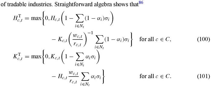
Example 3.2.1 is extreme because it assumes all industries are nontradable. Assume instead that T_t = 0, and let Iⁿ = N_t ∩ I_c,_t. As a result of agglomeration effects, any collection of sets Iⁿ (with Iⁿ = 0 for all c ∈ C) that constitutes a partition of N_t is an equilibrium of the world economy. Let again H^t_t and K^_t be the factor endowments used in the production of tradable goods, i.e. all final goods and the intermediate inputs of tradable industries. It follows that^[322]

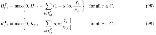
Equations (98) and (99) show the factor supplies that are left after subtracting from aggregate factor supplies the factors used in nontradable industries. These equations are analogous to Equations (87) and (88) of Section 3.1. One can use Equations (98) and (99) and a given collection of sets I_c^N_t to generalize the theory of Sections 2.4 and 2.5. For instance, in Example 2.4.1 Equations (47)-(52) still apply provided that we write H^t_t and K_cT_t instead of H_ct and K_ct.

The effects of this generalization of the theory are hard to assess given the multiplicity of equilibria and the inherent difficulty of finding a “respectable” selection criteria.^[323] It is always possible to find perverse equilibria in which regions specialize in the “wrong” industries, i.e. industries in which they do not have comparative advantage. Naturally, all the equilibria of Section 2 in which regions specialize in the industries in which they have comparative advantage still apply if requirement (R3) is not binding (as we have assumed so far). But there is no compelling reason to choose them over some of the alternatives. Moreover, if requirement (R3) is violated or is binding, the equilibria studied in Section 2 no longer apply to this world economy. The following example, inspired by Krugman and Venables (1995), relaxes the assumption that industries are “small” and clearly illustrates this point:

Example 3.2.2. Consider a world with two industries I = {A, M} and two regions C = {N, S}. Assume that both industries have the same factor intensities, i.e. α_i = α for all i ∈ I, but different sizes σA < 0.5 < a_M (remember that σA+o_m = 1). Also assume that both regions are identical, i.e. they have the same savings, human capital, industry productivities and initial condition. Assume next that the world starts in autarky and globalization proceeds in two stages: in the first one industry A becomes tradable, i.e. N_t = {M} for 0 ≤ t < T; and in the second stage also industry M becomes tradable, i.e. N_t = 0 for t '≥ T. In the world of autarky, both regions have the same income and the question that I shall address here is: How does globalization affect the world income distribution?

At date t = 0, all transport costs disappear except for those that affect the interme­diate inputs of industry M. There are two possible patterns of production and trade that can emerge as a result of this. The first one consists of both regions producing the same they did in autarky and not trading between them. Since both regions would have the same goods and factor prices, there would be no incentive for any producer to deviate from this equilibrium.^[324] The second possible pattern of production and trade that can emerge consists of each region specializing in a different industry. For instance, assume N specializes in industry M. The absence of other local producers in industry M means that producers in S have no incentive to produce in industry M. Since spending on in­dustry M is more than half of world spending, factor prices are higher in N and therefore producers in N cannot compete in industry A.^[325]

It follows from this discussion that the first stage of globalization generates world in­equality and world instability. In the world of autarky, both regions had the same income level and income volatility was driven by volatility in fundamentals, i.e. savings, human capital and industry productivities. Globalization generates divergence in incomes be­cause in the equilibrium with specialization the region that “captures” industry M has higher income than the region that is “stuck” producing in industry A. The world income distribution is determined by Equation (97). One effect of this inequality is faster phys­ical capital accumulation in N than in S. Globalization also generates instability, since the pattern of specialization can now change capriciously just as a result of a change in expectations. At any time the specialization pattern can change to the detriment of N and to the advantage of S. This constitutes an additional source of income volatility that goes beyond fundamentals.

At date t = T, transport costs for the intermediate inputs of industry M vanish. Although the pattern of production and trade is not uniquely determined, we know that factor prices and incomes are uniquely determined.^[326] Moreover, since we have assumed that both industries have the same factor intensities, the world income distribution is now given by Equation (70). It follows that the second stage of globalization starts a slow process of convergence in incomes that eventually restores equality across regions. Throughout this process, expectations no longer play any role and the only sources of income volatility are fluctuations in fundamentals.

This example features a combination of agglomeration effects and “large” industries that underlies most of the work known as economic geography.^[327] This research has focused on explaining how income differences can arise among regions that initially have the same fundamentals. The view of globalization and development that arises from this literature is colorful and suggestive, although it has not been subjected yet to serious empirical analysis.

Not surprisingly, globalization might lead to a Pareto-inferior outcome in the world of this section. The following example, which is related to Examples 2.1.2 and 3.1.3, shows this:

Example 3.2.3. Consideraworldeconomywith H -and K -industries, such that I^h U I^k = I and I^h ∩ I^k = 0. Assume α_i = O if i ∈ I^h and α_i = f if i ∈ I^k, and β_i is small (but not zero) for all i ∈ I. Within each type there are “advanced” and “backward” industries. A-regions have the highest possible productivity in all industries, regardless of whether they are “advanced” or “backward”. B-regions have the highest possible productivity only in “backward” industries. Assume next that after globalization all industries are nontradable. This world is just a special case of Example 3.2.1. We know therefore that there is an equilibrium in which A-regions specialize in “backwards” industries while B-regions specialize in “advanced” industries. This equilibrium can be easily shown to deliver equal or less income and welfare than autarky. Since β_i is small for all i ∈ I, the benefits from an increase in market size are negligible. Since the allocation of production worsens relative to autarky, production and income go down as a result of globalization. Therefore, it is not possible to find a transfer scheme that ensures that globalization benefits all.^[328]

Although this is real a theoretical possibility, it is not clear yet how seriously should we take the possibility that globalization worsens the world allocation of production and reduces welfare. How important empirically are these agglomeration effects? What is the relative importance of randomness and comparative advantage in determining the pattern of production and trade? The answers to these questions are critical in deter­mining whether the basic policy prescription that simply opening up to trade leads to development really applies or not. In the worlds of this section, opening up to trade can lead to miracles and disasters alike. A miracle is nothing but a lucky region that attracts a large number of industries exhibiting agglomeration effects. A disaster is an unlucky region that cannot do so. Opening up to trade is therefore a gamble. It opens the door for industries to come into the region and enrich it, but it also opens the door for in­dustries to leave the region and impoverish it. Naturally, the temptation to change the odds of this gamble using industrial policies and protectionism might be overwhelming. The prescriptions for development are therefore easy to spot but not pleasant. This is a world characterized by negative international spillovers and strong temptations to use “beggar-thy-neighbor” policies.

What about market-size effects? In the world of Section 3.1, differences in regional market size played no role in determining the world income distribution. If intermediate inputs are tradable, all regions use the same specialized inputs and enjoy the same level of industry specialization or technology to produce final goods. In the world of this subsection, differences in regional market size can play a role in determining the world income distribution by allowing large regions to achieve a higher degree of industry specialization.^[329] This is one possible mechanism through which market size matters. The next section depicts a world in which market size effects become central.

3.3. The role of local markets

We turn next to a world in which the costs of trading intermediate inputs and final goods are prohibitive if i ∈ N_t, but negligible if i ∈ T_t. As in all the worlds considered in this chapter, the benefits of developing specialized inputs depend on the size of the indus­try’s market. For tradable industries, this market is the world economy. For nontradable industries, this market is the region. As a result, regional differences in market size will be translated into regional differences in the degree of specialization or technology of nontradable industries.^[330]

Formally, this model is very similar to the one in Section 3.1. Equations (81) and (82) describe investment and consumption, while Equations (83) and (84) still provide the numeraire rule and the price level. Naturally, Equation (3) describing spending patterns still applies to all regions, and Equations (5) and (6) describing technology apply to all regions, with the corresponding factor prices and industry productivities. The only difference with the model of Section 3.1 is when Equations (7)-(10) describing pricing policies, input demands and the free-entry condition apply. For tradable industries, these equations apply only to those regions where the lowest-cost producers are located. For nontradable industries, these equations apply to all regions and not only to the lowest- cost ones. Thus, Equation (44) no longer applies to producers in nontradable industries, and Equation (93) must be replaced by Equation (95). Market clearing conditions are also the same as in the model of Section 3.1, and consist of Equations (45) and (46) describing market clearing in regional factor markets, Equation (11) describing market clearing in global markets for tradable industries, and Equation (85) describing market clearing in regional markets for nontradable industries.

This completes the formal description of the model. For any admissible set of capital stocks, i.e. K_c0 for all c ∈ C, sequences for the vectors of savings, human capital and industry productivities, i.e. S_ct, H_ct and A_cit for all c ∈ C and for all i ∈ I, and a sequence for the set N_t (or T_t); an equilibrium of the world economy after globalization consists of a sequence of prices and quantities such that the equations listed above hold in all dates and states of nature. Like other worlds we have studied up to now, there might be multiple geographical patterns of production that are consistent with world equilibrium. But unlike the world of the previous subsection (and like the worlds of Section 2 and Section 3.1), prices and world aggregates are uniquely determined.

In this world economy, the set FPE_t is empty. Since intermediate inputs that are pro­duced in a region cannot be used in another region, the world economy cannot reach the level of efficiency of the integrated economy.^[331] Despite this, it is relatively straight­forward to analyze this world. Define again H_c^τ_t and as the factor endowments devoted to the production of tradable goods, i.e. all intermediate inputs and final goods

Since factor supplies are well behaved, all the results in Sections 2.4 and 2.5 regarding market-based incomes and factor prices still go through in the presence of nontradable industries. As in Section 3.1, the only important difference between the world of this subsection and the one in Section 2 is that there is a discrepancy between market-based and real incomes and factor prices. In particular, we can write the price level of region c as follows,

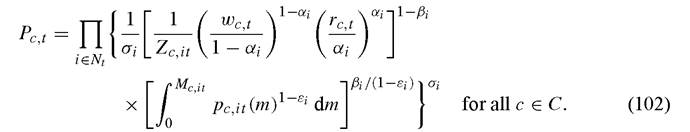
The only difference between this equation and Equation (91) is that the number and price of intermediate inputs varies across regions. Using Equations (6) and (10), we can transform Equation (103) into the following

Basically, this model brings another element to the theory of the price level. To the extent that nontradable industries exhibit increasing returns, regions with larger markets have lower price levels and higher real incomes.

It is straightforward to re-do some of the previous examples in the context of this world. But I shall not do this. The picture that this world generates is clear and unap­pealing from an empirical standpoint: regional differences in market size are reflected in regional differences in price levels. Ceteris paribus, larger local markets do not lead to higher market-based incomes and factor prices. But they do lead to lower price levels and, as a result, to higher real incomes and factor prices. This is clearly counterfactual.

^[1] To see this, note that the shares of human and physical capital devoted to producing the final good of the ith nontradable industry are now (1 - αi) and ů. Add over industries and note that the share of spending in the ith industry is σi Y^t ∙

4.