DATA AND METHODOLOGY

The present study uses the annual data on credit and deposit (both in current values) of the sched­uled commercial banks situated in different states published by The Reserve Bank of India.

Primarily we have applied the graphical tools for representing our data on credit deposit (C/D) ratio and credit share of each of the states over time where the latter is computed by the amount of credit of any state in a year divided by the ag­gregate credit of the sixteen states taken together as they cover around 75 per cent of the total credit in India. Since we have time series data for 37 year points the series may suffer from unit root problem or the series may not be stationary. Our analysis of causality tests between C/D ratio and credit share needs regression analysis and the regression of two non stationary time series variables give spurious results. Hence, we need basic time series exercises to be done.

In this paper we have used two different econo­metric methodologies, which are described briefly as follows. Section 4.1 discusses the econometric methodology of Granger Causality Test (GCT) and Section 4.2 fully describes the procedures of unit root test and cointegration and related error correction model (ECM).

The Methodology of GCT

In this section we describe the methodology of GCT that we have used in the present study (Granger (1969), Hamilton (1994)). The GCT is a statistical technique that helps to detect the nature of causality between two variables X_t and Y_t that may be present in a given time series data set on the variables. Application of the test requires the time series of the concerned variables to be stationary. Thus, it is necessary to examine first whether the time series of the variables are stationary or not. In case they are found non-stationary, they are transformed into stationary series by successive differencing until the differenced series become stationary. The augmented Dickey-Fuller (ADF) and Phillips-Perron (PP) unit root tests are used to test for presence of unit root in the original (level)∕differenced time series of the variables to ascertain the required stationarity. The GCT for a pair of non-stationary (integrated of order 1) variables X and Y is performed by estimating the following pair of autoregressive distributed lag regression equations:

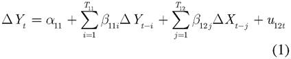
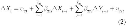
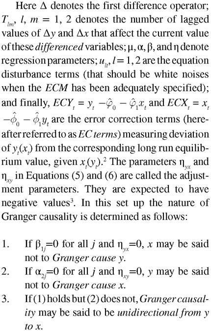
Here ∆ denotes the difference operator, Y_t and X_t denote the values of the variables X and Y at time t, respectively, T’s denote the number of lags, α's and β's denote regression parameters, and u_ts denote the equation disturbances.

The null hypothesis that X_t does not cause Y_t is rejected, if H₀: β_12j=0, for all j is rejected. Analogously, rejection of the null hypotheses H₀: β_22j=0 for all j signifies that Y_t does not cause X_t. F tests are performed to test these hypotheses.

The GCT gives rise to one of the following four conclusions:

1. X causes Y, but Y does not cause X,

2.

3. Both X and Y cause each other, and finally

4. Neither X causes Y nor Y causes X.

While (1) and (2) are cases of unidirectional causality, (3) and (4) correspond to bidirectional causality and absence of causality, respectively.

Unit Root Test

As already mentioned in above section of this paper we have examined whether credit deposit ratio - credit share data for different states were cointegrated using the Engle-Granger (1987) bivariate cointegration analysis framework and es­timated ECM for each state for which cointegration was observed to be significant, using econometric techniques appropriate for these data set¹. The econometric exercise involved three steps. In the first step, the unit roots test was performed for all the states’ series of credit-deposit ratio and credit share to ascertain whether or not the time series of the variables contained stochastic trend. In the second step, cointegration of credit deposit ratio and credit share series for all the states was examined. Finally, in the third step, the ECM was estimated for those states for which cointegration of credit deposit ratio and credit share had been found.

In the first step test procedure was used to test the presence of unit root in the time series data sets for individual states. The same procedure was also used in the second step while performing the Engle-Granger bivariate cointegration analysis. Finally, the third step was estimated by using ECM technique.

Unit Root Test

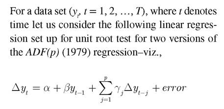
for the without time trend case and

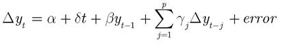
for the with time trend case.

Co-Integration Test

Given a data set on two variables (y, x) the single equation cointegration test proceeds as follows: First, the linear regression equation y_t = βx_t + U_i is estimated separately for individual state and the estimated regression residuals given by the following equation

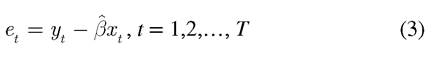
are obtained, where β 's denote the estimated parameters of the regression equation for each state.

Next, for each state the following ADF (p) equation is estimated:

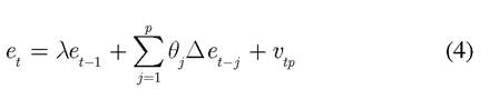
where ν is the equation disturbance term assumed to be a white noise. Methodology of cointegration test for the set of variables under consideration thus involves the test of unit root for the regression residuals {e_t} i.e., the null hypothesis H₀: λ=1 (i.e., no cointegration) is tested against the alternative hypothesis H₁: λConversely, if (1) does not hold but (2) does, Granger causality may be said to be unidirectional from x to y.

5. If both (1) and (2) do not hold, Granger causality between x and y may be said to be bi- directional.

6. If both (1) and (2) hold, Granger causality between x and y may be said to be absent (see Enders (1995), Glasure and Lee (1997) and Asafu-Adjaye (2000) for details).

In the present exercise, Equations (5) and (6) were estimated separately for each state. State­specific inference about the nature of Granger causality between x and y were then drawn by performing appropriate test of hypothesis for the relevant parameters of model, as laid down above.