THE DIVIDEND DISCOUNT MODEL
Several methods of fundamental common stock analysis have been devised over the years, but few match the intuitive appeal of regarding the stock price as the discounted value of expected future dividends.
This approach is analogous to the yield-to-maturity calculation for a bond and therefore facilitates the comparison of different securities of a single issuer. Additionally, the method permits the analyst to address the uncertainty inherent in forecasting a noncontractual flow1 by varying the applicable discount rate.To understand the relationship between future dividends and present stock price, consider the following fictitious example: Tarheel Tobacco’s annual common dividend rate is currently $2.10 a share. Because the company’s share of a nonexpanding market is neither increasing nor decreasing, it will probably generate flat sales and earnings for the indefinite future and continue the dividend at its current level. Tarheel’s long-term debt currently offers a yield of 10%, reflecting the company’s credit rating and the prevailing level of interest rates. Based on the greater uncertainty of the dividend stream relative to the contractual payments on Tarheel’s debt, investors demand a risk premium of four percentage points—a return of 10% + 4% = 14%—to own the company’s common stock rather than its bonds.
The stock price that should logically be observed in the market, given these facts, is the price at which Tarheel’s annual $2.10 payout equates to a 14% yield, or algebraically:
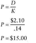
where P = Current stock price
D = Current dividend rate
K = Required rate of return
If the analyst agrees that 14% is an appropriate discount rate, based on a financial comparison between Tarheel and other companies with similar implicit discount rates, then any price less than $15 a share indicates that the stock is undervalued.
Alternatively, suppose the analyst concludes that Tarheel’s future dividend stream is less secure than the dividend streams of other companies to which a 14% discount rate is being applied. The analyst might then discount Tarheel’s stream at a higher rate, say 15%, and recalculate the appropriate share price as follows: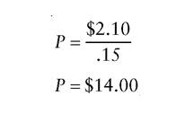
A market price of $15 a share would then indicate an overvaluation of Tarheel Tobacco.
Dividends and Future Appreciation
size=2 color=black face="Times New Roman">When initially introduced to the dividend-discount model, many individuals respond by saying, “Dividends are not the only potential source of gain to the stockholder. The share price may rise as well. Shouldn’t any evaluation reflect the potential for appreciation?” It is in responding to this objection that the dividend-discount model displays its elegance most fully. The answer is that there is no reason for the stock price to rise in the future unless the dividend rises. In a no-growth situation such as Tarheel Tobacco, the valuation will look the same five years hence (assuming no change in interest rates and risk premiums) as today. There is consequently no fundamental reason for a buyer to pay more for the stock at that point. If, on the other hand, the dividend payout rises over time (the case that immediately follows), the stock will be worth more in the future than it is today. The analyst can, however, incorporate the expected dividend increases directly into the present-value calculation to derive the current stock price, without bothering to determine and discount back the associated future price appreciation. By thinking through the logic of the discounting method, the analyst will find that value always comes back to dividends.
Valuing a Growing Company
No-growth companies are simple to analyze, but in practice most public corporations strive for growth in earnings per share, which, as the ensuing discussion demonstrates, will lead to gains for shareholders.
In analyzing growing companies, a somewhat more complex formula must be used to equate future dividends to the present stock price: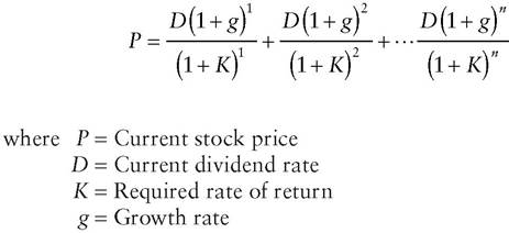
A number of dollars equivalent to P, if invested at an interest rate equivalent to K, will be equal, after n periods, to the cumulative value of dividends paid over the same interval, assuming the payout is initially an amount equivalent to D and increases in each period at a rate equivalent to g.
Fortunately, from the standpoint of ease of calculation, if n, the number of periods considered, is infinite, the preceding formula reduces to the simpler form:
![]()
In practice, this is the form ordinarily used in analysis, since companies are presumed to continue to operate as going concerns, rather than to liquidate at some arbitrary future date.
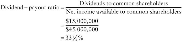
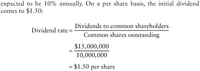
Figures projected from the financial statements of the fictitious Wolfe Food Company (Exhibit 14.1) illustrate the application of the dividenddiscount model. Observe that the company is expected to pay out 33 1/3% of its earnings to shareholders in the current year:
If Wolfe maintains a constant dividend-payout ratio, it follows that the growth rate of dividends will equal the growth rate of earnings, which is
EXHIBIT 14.1 Selected Financial Data for Wolfe Food Company
Net income available to common shareholders $45,000,000
Dividends to common shareholders $15,000,000
Common shares outstanding 10,000,000
Expected annual growth in earnings 10%
Investors’ required rate of return, given predictability of Wolfe’s earnings 13%
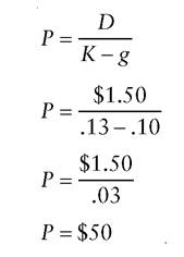
With these numbers, the analyst can now use the valuation formula to derive a share price of $50 for Wolfe:
The execution of this model rests heavily on the assumptions underlying the company’s projected financial statements. To estimate the future growth rate of earnings, the analyst must make informed judgments both about the growth of the company’s markets and about the company’s ability to maintain or increase its share of those markets.
Furthermore, the company’s earnings growth rate may diverge from its sales growth due to changes in its operating margins that may or may not reflect industrywide trends.Because of the uncertainties affecting such projections, the analyst should apply to equity valuation the same sort of sensitivity analysis discussed in connection with financial forecasting (see Chapter 12). For instance, if Wolfe Foods ultimately falls short of the 10% growth rate previously projected, then the $50 valuation will prove in retrospect to have been $12.50 too high:
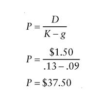
Therefore, an analyst whose forecast of earnings growth has a margin of error of one percentage point should not put a strong “Buy” recommendation on Wolfe when it is trading at $45 a share. By the same token, a price of $25, which implies a 7% growth rate, can safely be regarded as an undervaluation, provided the other assumptions are valid.
Earnings or Cash Flow?
Intuitively app ealing though it may be, the relating of share price to future dividends through projected earnings growth does not jibe perfectly with reality. In particular, highly cyclical companies do not produce steady earnings increases year in and year out, yet the formula P = D/K-g demands a constant rate of growth. If, as assumed previously, the company’s dividendpayout ratio remains constant, the pattern of its dividends will plainly fail to fit neatly into the formula.
What saves the dividend-discounting approach from irrelevance is that companies generally do not strive for a constant dividend-payout ratio at all costs. More typically, they attempt to avoid cutting the amount of the payout, notwithstanding declines in earnings.
For example, a company that aims to pay out 25% of its earnings over a complete business cycle might record a payout ratio of 15% in a peak year and 90% or 100% in a trough year. Indeed, a company that records net losses may maintain its dividend at the established level, at least for a few years, resulting in a meaningless payout-ratio calculation. (If losses persist, financial prudence will usually dictate cutting or eliminating the dividend to conserve cash.) As a rule, a cyclical company will not increase its dividend on a regular, annual basis. Nevertheless, the board will ordinarily endeavor to raise the payout over the longer term. In all of these cases, the P = D/K-g formula will work reasonably well as avaluation tool, with the irregular pattern of dividend increases recognized through adjustments to the discount rate (K).
Although the dividend-discount model can accommodate earnings’ cyclicality, the analyst must pay close attention to the method by which a company finances the continuation of its dividend at the established rate. A chronically money-losing company that borrows to pay dividends is simply undergoing slow liquidation. (It is replacing its equity, 100% of it in time, with liabilities.) In such circumstances, the key assumption that dividends will continue for an infinite number of p eriods becomes unsustainable.
On the other hand, a cyclical company may sustain losses at the bottom of a business cycle but never reach the point at which its funds from operations, net of capital expenditures required to maintain long-term competitiveness, fail to cover the dividend. Maintaining the dividend under these circumstances poses no financial threat. Accordingly, many analysts argue that cash flow, rather than earnings, is the true determinant of dividendpaying capability. By extension, they contend that projected cash flow, rather than earnings-per-share forecasts, should be the main focus of equity analysis.
Certainly, analysts need to be acutely conscious of changes in a company’s cash-generating capability that are not paralleled by changes in earnings.
For example, a company may for a time maintain a given level of profitability even though its business is becoming more capital-intensive. Rising plant and equipment requirements might transform the company from a self-financing entity into one that is dependent on external financing. Return on equity will not reflect the change until, after several years, either the resulting escalation in borrowing costs or the increase in the equity base required to support a given level of operating earnings becomes material. Furthermore, as detailed in Chapters 6 and 7, reported earnings are subject to considerable manipulation. In fact, that is the flaw that help ed to popularize the use of cash flow analysis in the first place. Cash generated from operations, which is generally more difficult for companies to manipulate than earnings, can legitimately be viewed as the preferred measure of future dividend-paying capability.Notwithstanding these arguments, earnings per share forecasts remain the focal point of equity research on Wall Street and elsewhere. (As explained in Chapter 3, some companies have managed to shift analysts’ focus from GAAP earnings to so-called pro forma earnings.) For many companies, the components of cash flow other than net income, especially depreciation, are highly predictable over the near term. By accurately forecasting the more variable component, earnings, an investor can get a fairly good handle on cash flow as well. To some extent, too, the unflagging focus on earnings probably reflects institutional inertia. Portfolio managers measure the accuracy of brokerage houses’ equity analysis in terms of earnings per share forecasts and investment strategists rely on aggregate earnings per share forecasts to gauge the attractiveness of the stock market as a whole. Analysts who lack an EPS forecast simply have a hard time getting into the discussion. Despite the stranglehold of earnings forecasts, however, a mechanism is available for adjusting a stock evaluation when the quality of the forecasted earnings is questionable. Investors can reduce the earnings multiple, as explained in the following section.