WHY P/E MULTIPLES VARY
Justifications for differences in earnings multiples derive from the variables of the preceding valuation formulas. Consider the following two equations:
![]()
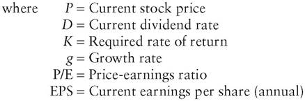
Substituting D/K - g, which equals P, for the P in the other equation, produces the following expanded form:
Using this expanded equation permits the analyst to see quickly that an increase in the expected growth rate of earnings produces a premium multiple.
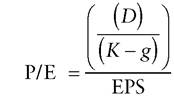
For example, both Wolfe Food Company and Grubb & Chao have 10% growth factors, and both stocks currently trade at 11.1 times earnings. Suppose another competitor, Eatmore & Co., can be expected to enjoy 11% growth, by virtue of concentration in faster-growing segments of the food business. A substantially higher multiple results from this modest edge in earnings growth: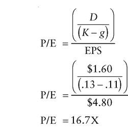
Eatmore & Co.’s earnings will not, however, command as big a premium (16.7X vs. 1.1 X for its competitors) if the basis for its higher projected growth is subject to unusually high risks. For example, Eatmore’s strategy may emphasize expansion in developing countries, where the rate of growth in personal income is higher than in the more mature economy of the United States.
If so, Eatmore may be considerably more exposed than Wolfe or Grubb & Chao to the risks of nationalization, new restrictions on repatriation of earnings, protectionist trade policies, and adverse fluctuations in exchange rates. If so, the market will raise its discount rate (K) on Eatmore’s earnings. An increase of just one-half percentage point (from 13.0% to 13.5%) wipes out more than half the premium in Eatmore’s multiple, dropping it from 16.7X to 13.3X:
In effect, the ability to vary the discount rate, and therefore to assign a lower or higher multiple to a company’s earnings, is the equity analyst’s defense against the sort of earnings manipulation by management described in Chapter 3. A company may use liberal accounting practices and skimp on long-term investment spending, yet expect the resulting artificially inflated earnings per share to be valued at the same multiple as its competitor’s more legitimately derived profits. Indeed, the heart of many management presentations to analysts is a table showing that the presenting company’s multiple is low by comparison with its peers. Typically, the chief executive officer cites this table as proof that the company is undervalued. The natural corollary is that in time investors will become aware of the discrepancy and raise the multiple, and therefore the price of shares owned by those who are astute enough to buy in at today’s dirt-cheap level.
These stories are sometimes persuasive, yet one must wonder whether such “discrepancies” in earnings multiples are truly the result of inattention by analysts. In the case of a large-capitalization company, hundreds of Wall Street and institutional analysts probably are making the comparison on their own. If so, they are fully aware of the below-average multiple but consider it justified for one or more reasons, including the following:
■ The company’s earnings are more cyclical than those of its peer group.
■ The company has historically been prone to earnings “surprises,” which raise suspicions that the reported results reflect an exceptionally large amount of “earnings management.”
■ Management has a reputation for erratic behavior (e.g., abrupt changes in strategy, ill-conceived acquisitions) that makes future results difficult to forecast.
Analysts may be mistaken in these perceptions, and may genuinely be undervaluing the stock.
The low multiple is a conscious judgment, however, not a function of neglect. Even a small-capitalization company, which can more credibly claim that its stock is underfollowed by Wall Street, may have the multiple it deserves, although its competitors sport higher P/E ratios. It is appropriate to assign an above-average discount factor to the earnings of a company that competes against larger, better-capitalized firms. A small company may also suffer the disadvantages of lack of depth in management and concentration of its production in one or two plants.Recognizing that qualitative factors may depress their multiples, companies often respond in kind, arguing that their low valuations are based on misperceptions. For example, a company in a notoriously cyclical industry may argue that it is an exception to the general pattern of its peer group. Thus, a manufacturer of automotive components may claim that its earnings are protected from fluctuations in new car sales by a heavy emphasis on selling replacement parts. Whether or not consumers are buying new cars, the reasoning goes, they must keep their existing vehicles in good repair. In fact, sales of replacement parts should rise if the existing fleet ages because fewer individuals buy new autos. Similarly, a building-materials manufacturer may claim to be cushioned against fluctuations in housing starts because of a strong emphasis in its product line on the remodeling and repair markets.
These arguments may contain a kernel of truth, but investors should not accept them on faith. Instead of latching on to the “concept” as a justification for immediately pronouncing the company’s multiple too low, an analyst should independently establish whether an allegedly countercyclical business has in fact fit that description in past cycles. It is also important to determine whether the supposed source of earnings stability is truly large enough to offset a downturn of the magnitude that can realistically be expected in the other areas of the company’s operations.
A good rule to remember is that a company can more easily create a new image than it can recast its operations.
Analysts should be especially wary of companies that have tended to jump on the bandwagon of “concepts” associated with the hot stocks of the moment. During the late 1970s, skyrocketing oil prices led directly to higher expected earnings growth (g), and hence higher P/E multiples and stock prices for oil producers. Suddenly, chemical companies, capital-goods producers, and others began presenting themselves as “energy plays.” Some did so by acquiring oil properties, but others simply began publicizing their existing, albeit tangential, links to the oil business in markets that might conceivably have benefited from rising petroleum prices. A few years later, when oil prices collapsed, these same companies deleted from their annual reports the glowing references and photographs playing up their energy-relatedness. Around the same time, as the economic boom ended in Houston and other cities that had benefited from surging oil prices, national retailing chains became less vocal about their concentration in the Sunbelt, which had for several years been synonymous with high growth and therefore high P/E ratios.Normalizing Earnings
Companies have strong incentives to gain increases, however modest, in their earnings multiples, even at the cost of stretching the facts to the breaking point (or beyond). Accordingly, it is prudent to maintain a conservative bias in calculating appropriate multiples. In addition to upping the discount rate (K) when any question about the quality of earnings arises, the analyst should normalize the earnings per share trend when its sustainability is doubtful.
Suppose, for example, that the fictitious PPE Manufacturing Corporation’s earnings per share over the past five years are as shown in Exhibit 14.4. PPE has customarily commanded a multiple in line with the overall market,
EXHIBIT 14.4 PPE Manufacturing Corporation Earnings History Table
| Year | Earnings per Share |
| 2002 2003 2004 2005 2006 | $1.52 1.63 1.86 2.04 2.67 (Estimated) |
which is at present trading at 12 times estimated current-year earnings. By this logic, a price of 12 times $2.67, or approximately 32, seems warranted for PPE stock.
Exhibit 14.5 shows, however, that the current-year earnings estimate is well above PPE’s historical trend line, making the sustainability of the
EXHIBIT 14.5 PPE Manufacturing Corporation Earnings History Graph
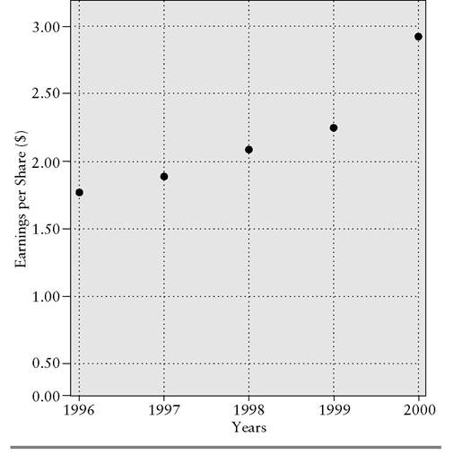
current level somewhat suspect.
As it turns out, the $2.67 estimate is bloated by special conditions that will probably not recur in the near future. Specifically, the customers for PPE’s major product are stepping up their purchases in anticipation of an industrywide strike later in the year. A temporary shortage has resulted, causing buyers to raise their bids. With its plants running flat out (reducing unit costs to the minimum) and its price realizations climbing, PPE is enjoying profit margins that it has never achieved before—and probably never will again.It hardly seems appropriate to boost PPE’s valuation from 24½ (12 times last year’s earnings per share) to 32, a 31% increase, solely on the basis of an EPS hiccup that reflects no change in PPE’s long-term earnings power. Accordingly, the analyst should normalize PPE’s earnings by projecting the trend line established in preceding years. Exhibit 14.6 shows such a
EXHIBIT 14.6 PPE Manufacturing Corporation Earnings Trend—Least-Squares Method
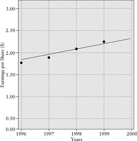
projection, using the least-squares method. The formula for this method is as follows:
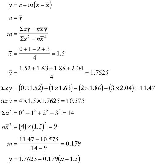
Solving for x = 4, we derive a current-year trend-line value of $2.21. Applying the market multiple of 12 produces an indicated stock price of 26½. Some modest upward revision from this point may be warranted, for if nothing else the company can reinvest its windfall profit in its business and generate a small, incremental earnings stream. By no means, though, should the company be evaluated on the basis of an earnings level that is not sustainable.
Sustainable Growth Rate
Sustainability is an issue not only in connection with unusual surges in earnings, but also when it comes to determining whether a company’s historical rate of growth in earnings per share is likely to continue.
The answer is probably “no” if the growth has been fueled by anything other than additions to retained earnings per share.Consider the following derivation of earnings per share:
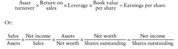
Earnings per share will not grow merely because sales increase. Any such increase will be canceled out in the preceding formula, since sales appears in the denominator of return on sales as well as in the numerator of asset turnover. Only by an increase in one of the four terms on the left side of the equation, or by a reduction in the number of shares outstanding, will the product (earnings per share) rise. Aggressive management may boost asset turnover, but eventually the assets will reach the limits of their productive capacity. Return on sales, likewise, cannot expand indefinitely because too- fat margins will invite competition. Leverage also reaches a limit because lenders will not continue advancing funds beyond a certain point as financial risk increases. This leaves only book value per share, which can rise unceasingly through additions to retained earnings, as a source of sustainable growth in earnings per share. As long as the amount of equity capital invested per share continues to rise, more income can be earned on that equity, and (as the reader can demonstrate by working through the preceding formula) earnings per share can increase.
A company’s book value per share will not rise at all, however, if it distributes 100% of its earnings in dividends to shareholders. (This, by the way, is why an immediate increase in the dividend-payout ratio will not ordinarily cause a direct, proportionate rise in the stock price, as might appear to be the implication of the equation P = D/K-g.) Assuming the company can earn its customary return on equity on whatever profits it reinvests internally, raising its dividend-payout ratio reduces its growth in earnings per share (g). Such a move proves to be self-defeating as both the numerator and the denominator (D and K-g, respectively) rise and P remains unchanged.
To achieve sustainable growth in earnings per share, then, a company must retain a portion of its earnings. The higher the portion retained, the more book value is accumulated per share and the higher can be the EPS growth rate. By this reasoning, the following formula is derived:
Substainable growth rate = (Return on equity) × (Income reinvestment rate)
where Income reinvestment rate = 1 - Dividend payout ratio
As mentioned, the one remaining way to increase earnings per share, after exhausting the possibilities already discussed, is to reduce the number of shares outstanding. During the 1990s, a number of companies used stock buybacks to maintain EPS growth in the face of constrained opportunities for revenue growth. Between 1995 and 1999, International Business Machines spent $34.1 billion to repurchase shares, more than its cumulative net income for the period of $31.3 billion. By reducing its shareholders’ equity through stock purchases, IBM increased its leverage and, therefore, its financial risk. Moreover, the company intensified this effect by adding to its debt. Financial commentator James Grant quipped that if IBM continued to buy in shares, it would undergo a slow-motion leveraged buyout.2 Such EPS-boosting plans tend to be self-limiting, for as already noted, lenders refuse at some point to countenance increased indebtedness.
Analysts should note one subtlety in calculating the impact of stock repurchases on earnings per share. To the extent that the company funds the buybacks with idle cash, the increase in EPS is offset by a reduction arising from forgone income on investments. If a company has far more cash on its balance sheet than it can employ profitably in its operations, it is unfair to accuse management of deceitfully inflating its per share income by buying in stock.