Consequences of non-logistic resource growth
Abrams (1980b) discussed the impact of non-logistic resource growth on competition. That article assumed the theta-logistic model (see Figure 5.1), in which the per capita growth rate declines at a rate proportional to the resource abundance (R) raised to the power θ.
Consumer competition coefficients that are independent of resource abundance only occur for the case of θ = 1 for all resources (i.e., logistic growth). Changes in either relative or absolute resource abundances alter the competition coefficients when θ = 1 for one or more resources. Figure 6.3 provides some examples of the response of consumer abundance to changes in one consumer’s mortality for simple 2-resource models with biotic resources, and with symmetric resource use by the two consumers (both have attack rate C on their ‘preferred’ resource and (1 - C) on the less preferred). In these cases, the contribution of a given resource to the competition coefficient (eq. (3.2)) changes depending on its abundance. The contribution increases with greater abundance when θ 1 (Abrams 1980b). Figure 6.3 spans the full range of d1 values allowing coexistence for the given d2. Because C > 1/2, a low mortality of consumer 1 (d1) means that resource 1 has low relative abundance, and therefore a high weighting in calculating the competitive effect in Figure 6.3A. Because consumer 1 has a threefold advantage in consumption rate on resource 1, its relative effect on consumer 2 (α21) is approximately three times that of consumer 1 on itself when resource 1 is rare. Conversely, when resource 2 is very rare, the effect on consumer 2 approaches 1/3. Thus, with θ = 2, as in Figure 6.3A, a low d2 means that consumer 2’s ‘preferred’ (higher C) resource is rare, so its impact on consumer 1 is largely determined by this resource. The reverse is true with θ = 1/2, as in Figure 6.3B; here a resource has a higher weighting when it is common; thus the lines giving the competition coefficients have opposite slopes in the two panels of Figure 6.3. It is important to remember that the θ-logistic is only one of many possible models of nonlinear density dependence (Chapter 5), and it is only being employed here because it is mathematically simple and is the most widely used nonlinear model.The potential for discontinuous change in the equilibrium abundance of a consumer in response to continuous change in its own or another consumer’s mortality rate is driven by extinction (or addition) of a resource. The mortality rate at which resource extinction (or addition) occurs is solely determined by the consumer growth equations in the models considered here, which lack any direct effect of consumer abundance on consumer per capita growth rate. This means that the mortality di required for resource extinction is not affected by the exponent describing resource density dependence. However, the question of whether extinction of one consumer occurs before the di of the manipulated species reaches the point of resource extinction is affected by θ. The lowest value of C (with C > 1/2) that can produce discontinuous change is smaller for larger values of θ. For the example of a MacArthur system (θ = 1) shown in Figure 3.2, if C is decreased, the discontinuity at the lower d1 disappears when C < 0.589, while for θ = 2, discontinuous change in consumer 2 at the lower d1 occurs until C < 0.5341. This means that discontinuous change occurs for
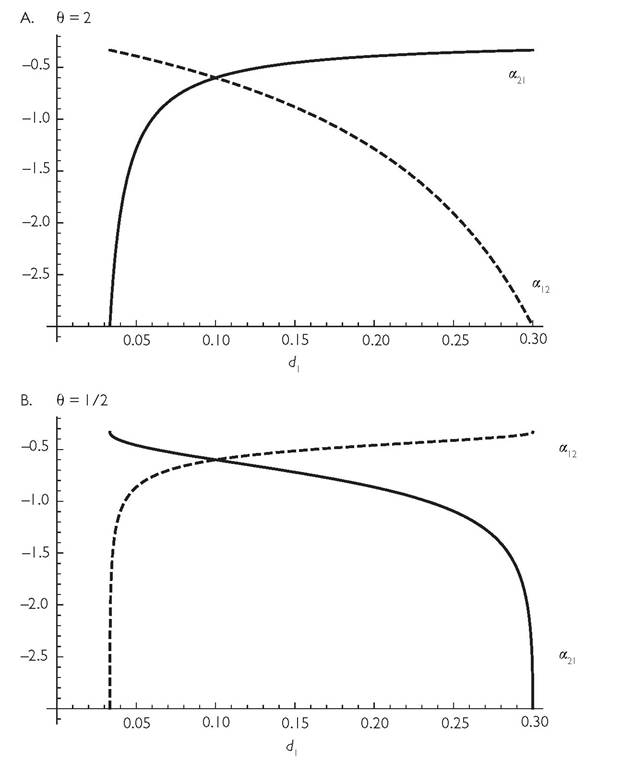
Fig. 6.3 'The effect of nonlinear resource density dependence (θ / 1) on the shape of consumercompetition as measured by eq. (3.2), for a range of different mortality rates of consumer species 1, d1, when d2 = 0.1.
The other parameters are; r = k = 1; and C = 3/4. In panel A, θ = 2, and in panel B, θ = 1/2. In both panels, the dashed line is α21, and solid is α12. The value of both competition coefficients using MacArthur’s formula is -0.6. The actual coefficients shown below only have that value when death rates are equal, (di = 0.1).a wider range of consumer similarities for resources having θ = 2 than for otherwise similar resources with θ = 1. More generally, the range of C producing discontinuous change in equilibrium consumer abundance in response to a continuous change in mortality expands with larger θ regardless of the initial value of this (positive) exponent.
Levine (1976) and Vandermeer (1980) showed that competition between resources in a 2-consumer system could produce mutually positive effects of each consumer species on the other. Both studies assumed the MacArthur model with the addition of direct and instantaneous linear competitive effects between resources. However, Levine did not consider cases in which resource species became extinct, and Vandermeer (1980) only examined equilibria, so did not examine the phenomenon of discontinuous change in abundance with continuous parameter change. This was extended to systems with type II consumer functional responses, including the possibility of large magnitude perturbations and resource exclusion by Vandermeer (2004, 2006), Abrams and Matsuda (2005), and Abrams and Nakajima (2007). The results in these works showed that the sign of the between-consumer effects often changed with the magnitude of the perturbation to the consumer. Abrams and Nakajimas (2007) results also confirmed the finding of Abrams (1998); i.e., the largest competitive effects on abundance frequently occur in cases with relatively low consumer similarity in resource uptake rates.
A second commonly used representation of resource growth is the chemostat model, which is routinely used to describe non-reproducing (abiotic) resources.
The consequences of having abiotic resources were known to be nonlinear competitive effects between two consumers as early as MacArthur (1972). MacArthur briefly considered resources that were externally supplied at a constant rate and only left the system by consumption (i.e., a chemostat with no loss of unconsumed resources). This model produces lower weighting of resources whose abundances are lower when calculating a competition coefficient. However, unlike biotic resources, externally supplied (abiotic) resources cannot be driven to extinction. Unfortunately, MacArthur (1972) did not treat this case in detail, and he instead stressed that competitive effects could be approximated by a linear model for abundances very close to the equilibrium point. Unfortunately, the effects of very small changes (in densities or neutral parameters) near an equilibrium point are seldom measurable, and are only of ecological significance if they reliably indicate the responses to larger magnitude changes. Schoener (1974c) showed that MacArthur’s abiotic resource model, with resources assumed to be at equilibrium led to extremely nonlinear competitive effects across the full range of competitor densities in a system where each consumer had one or more resource(s) that were not shared with the other consumer^). Abrams (1975) demonstrated that such models produced quite different magnitudes of the competition coefficient at equilibrium than those produced by an otherwise similar MacArthur model. Systems with abiotic resources that obey the full chemostat equation (which includes resource loss due to causes other than consumption) were later explored by Abrams (1977) and Schoener (1978); this again led to nonlinear competition when resources were assumed to reach a quasi-equilibrium with consumers. In all of these cases, the relative weighting of a particular resource in determining the competition coefficient is smaller when the resource is less abundant. Lowered mortality of a given consumer differentially depletes the resources it consumes at a higher rate, so these contribute less to its competitive effect(s) on the other consumer(s).The probability of resource exclusion increases with the number of resources. Analyses of 2- and 3-consumer systems with very many resources (Abrams et al. 2008a and Abrams and Rueffler 2009) showed that competition coefficients frequently increase with greater consumer differences in resource utilization. These studies used models with independent logistically growing resources having identical growth parameters. Abrams and Rueffler (2009) examined a model with three consumer species, and found that coexistence was impossible for some cases where the middle consumer had a resource utilization curve that was not exactly intermediate between the two other consumers. This result again required high enough consumer efficiency (e.g., low d) that resources used at a high enough rate by one or both species were driven extinct.
Pronounced nonlinearity of competitive effects was observed in some of the early experimental work on two-species competition (Ayala 1969; Gilpin and Justice 1972; Gilpin and Ayala 1973). Such nonlinearity was shown to be true of singlespecies growth (intraspecific competition) in many species by Pomerantz et al. (1980). These authors began their paper (p. 311) with the following statement: ‘The linearity assumption of the logistic model of population growth is violated for nearly all organisms’. The type of nonlinearity that arises in abiotic growth models usually leads to lower weights associated with rarer resource types when calculating expressions (3.1) or (3.2) from Chapter 3. (Recall that measure (3.2) is equivalent to the competition coefficient at equilibrium.) For other types of growth models, the nonlinearity in single resource growth should translate into nonlinearity of competitive effects between consumers of those resources. This makes it particularly puzzling that competition theory has retained its focus on the linear case.
6.4