Consequences of nonlinear functional responses

The model used in most of the preceding sections assumes linear functional respons­es of both consumer species, which was previously argued to be rare in nature and to have special properties.

(3.2) —is quite different when the MacArthur consumer-resource system is modified by adopting multi-species type II responses. Furthermore, there is actually a higher probability of resource exclusion in stable systems with type II responses (contrary to McPeek (2019a)), as shown in this section. Finally, the presence of cycles due to type II responses does not only affect consumer coexistence; it leads to a variety of inter­specific effects because perturbations to one consumer alter the nature and amplitude of cycles of all species. These effects were noted by Armstrong and McGehee (1980) and documented in more detail in Abrams and Holt (2002), Abrams et al.

Consequences of type II responses in stable systems are discussed in the first subsection 6.4.1 below, while the consequences of cycles are explored in 6.4.2.

6.4.1 Effects of nonlinear functional responses on consumer competition in systems with stable equilibria

A type II functional response alters the relationship between overlap in resource use and competition coefficients; it also changes most other possible measures of the strength of competition, even in systems that have stable equilibria Abrams (1980a). Type II responses also have a major effect on the nature of apparent competition between resources (Abrams et al. 1998).

The presence of a type II response in a system that is otherwise identical to the 2-consumer-2-resource MacArthur model of eqs (6.1a) significantly changes the relationship between similarity in resource use and the competition coefficient (eq.

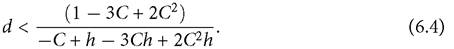
(3.2) ). Figure 6.4 assumes a symmetrical 2-consumer-2 resource system with two independent logistic resources, linear consumer numerical responses, and type II functional responses. Consumer 1 has attack rates of C and (1 - C) on resources 1 and 2 respectively, while consumer 2 has attack rates of (1 - C) and C. Thus overlap in utilization is 0 when C = 1 and overlap is 1 when C = 1/2. For any value of h > 1, a small enough d makes the equilibrium point unstable. The competition coefficient (eq. (3.2), when d₁ = d₂ = d) is:

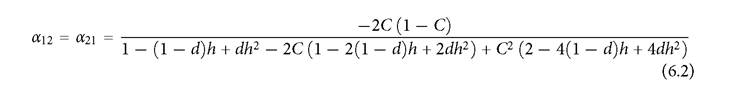
Equation (6.2) becomes independent of C and equals -1 when d = (h-1)∕(h(1 + h)).

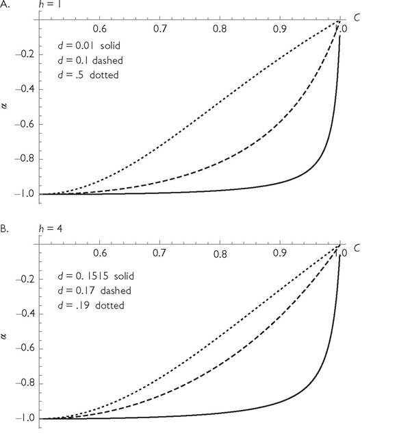
Fig. 6.4 The relationship between overlap, C, and the competition coefficient (α) in a symmet­ric 2-consumer-2-resource systems with type II functional responses having equal handling times, h, for all consumer-resource pairs (and r₁ = r₂ = k = 1), and attack rates of C and 1 - C for its more- and less-preferred resources. Thus, over the range shown, larger C implies less overlap in resource use. In panel A, h = 1, which gives a stable system for all mortali­ty rates, d, and a maximum d of 1. In panel B, h = 4, which yields a stable equilibrium for d > 0.15, and no positive equilibrium for d > 0.2. In both cases, lower death rates in stable systems result in a competition coefficient closer to unity over a wider range of overlaps.

no-handling-time interaction strength when the mortality rate is close to the max­imum that allows consumer persistence in the absence of competition.

Another consequence of type II functional responses is that the competition coef­ficients generally differ from each other in this system with perfectly symmetrical resource use parameters when the mortality rates of the two consumers differ (i.e., when their equilibrium abundances are unequal). It is possible to get a closed form expression analogous to eq. (6.2) for cases when d₁ = d₂. The two competition coef­ficients for the simple 2-resource system assumed in Figure 6.4A (h = 1) are plotted as a function of the mortality rate of consumer 1 in Figure 6.5, with low overlap in panel A, and moderate overlap in panel B. In both panels, the lines cross at the d₁ value that is equal to the (fixed) d₂; the competition coefficient at this point is always larger in magnitude than the value for a corresponding system with linear consumer functional responses (given by the blue line). The x-axis spans the full range of d₁ val­ues that allow coexistence; consumer 2 is extinct for d1 values lower than the range shown, and consumer species 1 is extinct for d₁ above that range. The (negative) per­individual impact of species 1 on 2 (i.e., α₂₁) is smaller in magnitude when species 2 is relatively common due to a high death rate of consumer 1; if the death rate of species 1 is decreased, its negative impact of species 2 (per unit change in d₁) becomes larger in relative magnitude, and even exceeds the magnitude of the change in the abundance of species 1 on itself (α₂₁ < -1).

The type II functional response is only one of a wide range of nonlinear multi­species functional response forms, as noted in Chapter 3. Even within the category of Holling type II responses, a multi-resource system may have multiple independent single-resource functional responses if the resources are present at different times, so that handling one resource type does not interfere with capturing others. Adaptive choice by the consumer will also change the relationship. Thus, the possibilities illustrated here represent a small fraction of what is likely to occur in natural systems.

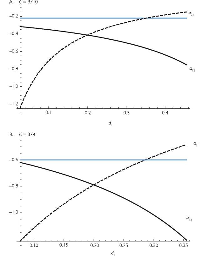
Fig. 6.5 The competition coefficients, αι₂, and α₂ι (eq. (3.2)) as a function of d₁ for d₂ = 0.2 in a 2-consumer-2-resource model with logistic resource growth and a type II con­sumer functional response with a handling time h = 1 for all consumer-resource pairs, and mirror image C values as in Figure 6.4. The blue line is the MacArthur formula for the product of the two α for linear functional responses; the dashed black line is α₂₁, and the solid black line is α₁₂. As d₁ increases, the competition coefficient of consumer 2 on 1 decreases, and that of consumer 1 on 2 increases.

The only one of the six focal articles discussed in Chapter 4 that gave explicit con­sideration to functional response shape was McPeek (2019a). However, even here, the claimed potential consequences do not include some that had been demonstrat­ed many years earlier. The one consequence of type II responses in stable systems claimed by McPeek (2019a) is a reduction in apparent competition in systems with a single consumer. McPeek (2019a, p. 1) states: ‘Saturating functional responses do not qualitatively alter the conditions for multiple consumers and resources to coexist at a stable point equilibrium, but do increase the range of apparent competitive abili­ties for resources that can invade and coexist’. Conditions for resource coexistence in single-consumer systems having type II functional responses were studied by Abrams et al. (1998) and Abrams (2009b, d). All of these works showed significant differences from the case of linear functional responses. However, they did not show a decreased likelihood of apparent competitive exclusion. As shown in more detail below, exclu­sion of resources in stable single-consumer systems is actually more likely in systems having type II functional responses than in otherwise comparable systems with linear responses.

In determining how functional response shape changes the range of parameter values allowing all resources to persist with one consumer, it is important to com­pare systems with equivalent consumer efficiencies (measured by the reduction in resource densities they bring about). Equivalent consumer efficiency is important because higher efficiencies strengthen apparent competition by increasing the con­sumer effects on all resources (Holt 1977). If type II functional responses (or higher handling times) implied lower efficiencies, species with such responses would be outcompeted. In general, the range of ‘apparent competitive ability’ of one resource species allowing coexistence with another is most appropriately measured by assess­ing the fraction of the total range of a neutral resource parameter of the focal species that allows coexistence with and without the competitor. The parameter r_i is the only neutral parameter in eqs (6.1a, b). Under a linear (MacArthur) model, an increase in r for one prey leads to a reduction in the equilibrium abundance of the other prey species in the presence of the single predator species. The range of relative mag­nitudes of r₁ and r₂ that allows resource coexistence in a system where C₁ = C₂ provides a measure of the breadth of conditions for apparent competitive coexis­tence. Another measure is provided by the fraction of the potential range of consumer mortality rate that allows coexistence of both resources when C₁ = C₂. Both of these potential range measures are examined below for 1-predator-2-prey systems and for 2-predator-2-prey systems, to determine how predator handling time affects the breadth of conditions under which prey coexist. It is shown that type II responses, and particularly those with greater handling time, should more often lead to appar­ent competitive exclusion of one of the two resources than in the corresponding linear response systems, at least when the systems are stable.

First consider the range of relative r-values allowing resource coexistence in a 1-consumer-2-resource system. This is a measure of coexistence bandwidth (Armstrong 1976) for resources, as r is a neutral parameter in the single-consumer version of eqs (6.1a), modified to have a handling time, h. Consider a simple case with r₁ = 1; C₁ = C₂ = 1/2; k₁ = k₂ = 1; and B₁ = B₂ = 1. The value of r₂ that is just large enough to cause extinction of resource 1 is given by

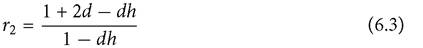
It is easily confirmed that this expression increases with h, seemingly suggesting that apparent competition is reduced. However, a comparison between systems with and without handling time should be characterized by similar effects of consumer pres­ence on the resources in both systems; i.e., equal equilibrium resource densities in the baseline case where r₁ = r₂. This can be achieved if d_t2 = d_t1/(1 + hd_t1), where the t1, t2 subscripts denote type I (linear) and type II (saturating) functional responses. Substituting the formula for d_t2 into expression (6.3) yields 1 + 2d_t1, which is the value of expression (6.3) for h = 0. Thus, 1-consumer-2-resource systems with type I and type II responses that have identical values of all parameters other than handling time are characterized by the same range of r values permitting coexistence of resources.

In the present analysis (and in McPeek, 2019a), the focus is on interactions between consumer species, so looking at the range of consumer mortalities allow­ing resource coexistence is more relevant than the range of r values of resources. Here I assume that the resources are characterized by equal r-values but unequal vul­nerabilities (C) to the consumer. The question is then, what fraction of the range of potential mortality rates (d) of the consumer results in exclusion of the higher- C resource. Using a 1-consumer-2-resource subsystem consistent with the previous 2-resource example (k_i = r_i = B_ij = 1; Cj ₁ + Cj₂ = 1), the maximum death rate that a predator with a linear functional response can sustain is d = 1. The maximum mortal­ity for a predator with a handling time h is d = 1∕(1+h). For example, if h = 1, d_max = 1/2, which is 1/2 the maximum for a linear response. I examine the d at which appar­ent competitive exclusion occurs with consumer 1 present when C₁₁ = C >1/2 and C₁₂ = 1 - C. Exclusion of resource 1 occurs when

If C = 3/4, for example, resource exclusion occurs for d ≤ 1/6 when h = 0, i.e., one-sixth of the maximum d (= 1) allowing consumer persistence. For the case of h = 1, exclusion (of the exclusive resource 1) occurs for d ≤ 1/7. This represents 2/7 of the maximum d of 1/2. Thus, apparent competitive exclusion is a more likely occurrence (occurs over a larger fraction of admissible d-parameter space; 2/7 rather than 1/6) when comparably efficient predators have saturating functional responses, rather than linear responses. Figure 6.6 compares the fraction of d parameter space

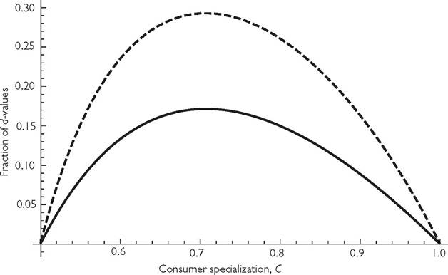
Fig. 6.6 The lines give the proportion of mortality (d) parameter space that yields extinction of the more vulnerable resource via apparent competition in a 1-consumer-2-resource model based on eqs (6.1a). The x-axis is the C-value of the more vulnerable resource (C₁ + C₂ = 1). Logistic resource growth is assumed with r = k = 1. The solid line assumes a type I functional response (h = 0), while the dashed line assumes h = 1. Handling times > 1 produce a larger fraction of admissible parameter space characterized by exclusion than does h = 1, but also allow for population cycles, which requires numerical analysis.

over which apparent competitive exclusion occurs for h = 0 and h = 1, for a system in which there are equal growth parameters of the two resources and C₁ + C₂ = 1. Within the range of handling times where all equilibria are stable (both lines in Figure 6.6), apparent competitive exclusion becomes more likely the greater the han­dling time. In the system examined here, the highest potential values of d in the parameter space are likely to imply extinction of a consumer species in a fluctuat­ing environment. Thus, the total realistic range of mortalities is likely to be smaller than implied by the deterministic model. As a result, the effective fraction of con­sumer mortality rates leading to resource exclusion is even larger than indicated in the figure. In systems that may exhibit cycles (h > 1 in this case), the exclusion con­ditions would have to be determined numerically when d is sufficiently low because of population cycles. This is illustrated in the following subsection.

6.4.2 Interactions in unstable systems with type II responses

It is useful at this point to illustrate the types of interactions that arise in models with biotic resources when nonlinear functional responses are considered in conjunction

Negativity, constancy, and continuity of competitive effects • 133 with resource exclusion and/or unstable equilibria. The results are again based on eqs (6.1b) above after modification by substituting multi-resource type II functional responses for the type I responses. Here, the analysis must be numerical. The nonlin­earity of the interaction can be illustrated by examining population sizes following different magnitudes of a press perturbation to a neutral parameter (per capita mor­tality, d will again be used below). The results provide examples of how population densities change with the mortality rate of one consumer, and how the resulting com­petition coefficient (eq. (3.2)) changes. A full exploration of parameter space for the model is beyond the scope of this work, but the examples presented are not excep­tional. They show a very complicated nonlinear response to a range of magnitudes of press perturbations applied to one of the competitors.

In these examples, the consumers each have a shared and an exclusive resource, and all resources have a very low rate of external immigration. Here the conversion efficiencies (Bif) are again set to unity, and the linear functional responses have been changed to type II responses with equal handling times (h = 2) for all consumer­resource pairs. Other parameters are given in the figure legends. In the two systems illustrated in Figure 6.7 and Figure 6.8 both consumers spend the majority of their time ‘handling’ resources when all resources are near carrying capacity. (Recall that ‘handling’ includes digestion.) The resource immigration rate keeps the resources from going extinct, but it is low enough to have minimal impact on equilibrium abundances.

Figure 6.7 examines competition in an example of the 3-resource system described in the previous paragraph. For both consumers the shared resource is character­ized by C = 1/3 and the exclusive resource by C = 2/3. The baseline mortality rate (d₁ = d₂ = 1/4) is low enough to produce unstable equilibria for most of the systems being plotted. (Other parameters are: r₁ = r₂ = r₃ = 2; K₁ = K₃ = 1; K₂ = 2; b_ij = 1; and d₂ = 0.25.) Panel A (which is identical to Figure 3.2 in Chapter 3) examines the competition coefficient α₂₁ (eq. 3.2) as a function of the mortality rate of consumer 1 (d₁). The line corresponds to an analysis based on the equilibrium points, while the dots are based on mean populations determined before and after a small (1%) change in d1. The two points characterized by the largest death rates in panel A are stable systems, which is why the point values describing the completion coefficient lie on the equilibrium line. Discontinuities in the equilibrium formula for the com­petition coefficient occur at four different points. Two of these (at d₁ = 1/8 and d₁ = 11/28) correspond to points at which one resource goes extinct, while the other two (at d1 = 1/20 and d1 = 13/44) are values for which a small increase in d1 has no effect on the equilibrium population size of consumer 1 making the denominator of eq. (3.2) zero. The corresponding MacArthur system (equal C_ij values, no handling time) yields α_ij = -1/3 for all cases. Panel B shows both the equilibrium (lines) and numerically determined mean densities (dots) of the consumers over the range of d₁ that allows persistence of consumer 1. Panel B also shows equilibrium resource abun­dances. There are many cases where the effect of a change in d1 on mean consumer densities has a sign opposite to that predicted by the equilibrium analysis, as well as cases where the effects on the mean and equilibrium population sizes differ greatly in magnitude.

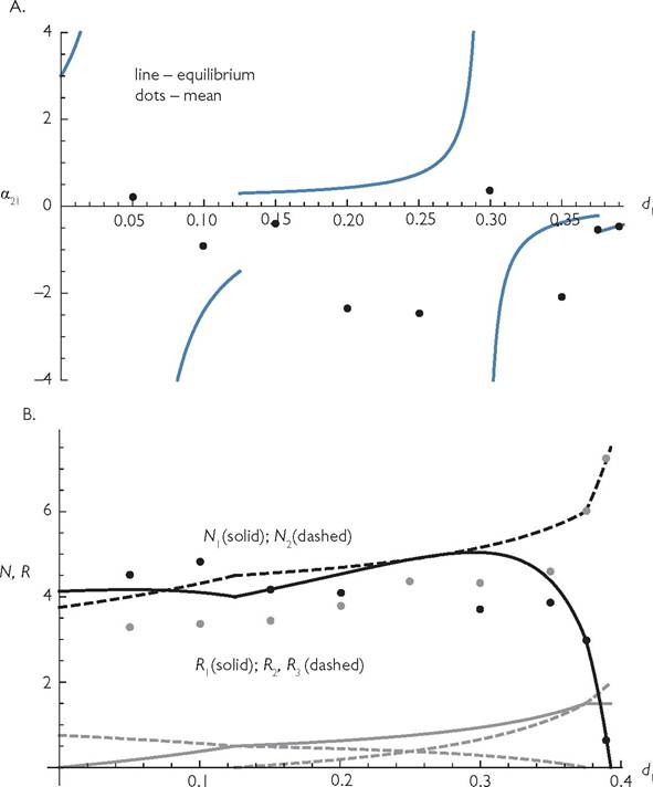
Fig. 6.7 (Note: Panel A is identical to Figure 3.2.)

A. 'The competition coefficient based on equilibrium densities (line segments) and mean den­sities (dots) for eqs (6.1b) modified by a type II response. The integrals determining the mean were evaluated for a selection of points spanning the range that allowed coexistence of the two species. Positive values of the point location mean that the two consumer species change in the same direction in response to increased death rate of species 1; they change in opposite directions for negative values. The parameter values are: r₁ = r₂ = r₃ = 2; k₁ = k₃ = 1; k₂ = 0.5; C₁₁ = 2/3; C₁₂ = 1/3; C₂₂ = 1/3; C₂₃ = 2/3; B_ij = 1; Ij = 0.00001; and d₂ = 0.25. Allhandlingtimes are h_ij = 2. This graph has four discontinuities corresponding to where a resource becomes extinct (d₁ = 0.125 and d₁ = 0.3928), and where greater mortality of consumer 1 does not alter its density, at d₁ = 0.05 and d₁ = 0.2954. The system exhibits cycles at all of the black points except for the two highest values.

B. The population densities of consumers and resources corresponding to panel A. The two black lines are the equilibrium densities of consumer 1 (solid) and consumer 2 (dashed). The mean densities of each consumer species corresponding to these lines are given by the dots for selected values of d₁ (grey dots for consumer 2 and black for consumer 1). The (lower) grey lines are the abundances of the three resources. The dashed lines are for resources 1 and 3, with the decreasing line corresponding to resource 3. The solid grey line is the density of resource 2.

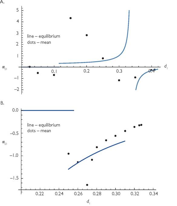
Fig. 6.8

A. The value of the competition coefficient (eq. (3.2)) based on both equilibrium densities (line) and actual mean densities (black dots), for a 2-consumer-3-resource system described by eqs (6.1b) modified to have multi-species type II responses. The parameter values for eqs (6.1b) are: r₁ = r₂ = r₃ = 2; k₁ = k₃ = 1; k₂ = 0.5; C₁₁= 0.9; C₁₂ = 0.6; C₂₂ = 0.6; C₂₃ = 0.9; and Bij = 1; The handling times (not shown in eqs (6.1b)) are h_ij = 2. Immigration of resource and baseline mortality are Ij = 0.00001 and d₂ = 0.3. Note that the abundance of consumer 1 is greater than that of consumer 2 at the value of d₁ = 0.3, where d₁ = d₂, even though the system is perfectly symmetrical for these values. There are two cyclic attractors here having asynchronous dynamics of the two species but reversed relative abundances; only one is represented here.

B. Competition in another shared-exclusive resource system; this one is identical to that illus­trated in Figure 6.7 except that the attack rates of the shared and exclusive resources have been reversed for both consumers; C₁₁ = 1/3, C₁₂ = 2/3, C₂₂ = 2/3, and C₂₃ = 1/3. The baseline mor­talities are 0.25 for both species; at this point the shared resource is extinct in the absence of immigration (and only present at very low levels given the resource immigration rate assumed here (as in Figure 6.7). This means that there is no competition. Competition occurs at d2 val­ues significantly above 0.25, and cycles characterize this range. The cycles allow both consumer species to persist above the value (d₁ = 0.30986) where species 2 would be predicted to go extinct assuming a stable equilibrium.

Figure 6.8 illustrates the competition coefficient α₂₁, as a function of d₁ for 3-resource models that differ slightly from those used in Figure 6.7. In Figure 6.8A, the relative use of the shared resource is higher for both competitors than in Fig­ure 6.7, and the absolute capture rates of all resources are also somewhat higher; C_exclusi_ve = 0.9 and C_sh_ared = 0.6. The figure also assumes somewhat higher baseline mortalities for both consumer species (d_i = 0.3). All other parameters are identical to those in Figure 6.7. The result for the corresponding MacArthur model without han­dling times would be a competition coefficient (eq. (3.2)) of-0.5455, regardless of the mortality rate, provided that the mortality rate did not cause resource exclusion. The results in Figure 6.8A again show a complicated pattern of change in α₂₁ with altered d₁. The lower discontinuity in the blue line corresponds to the lowest d₁ hav­ing a positive equilibrium for the shared resource. However, the shared resource is actually present for a range of d₁ values where the equilibrium is zero; this is due to population cycles. The black dots at mortalities of 0.05 and 0.1 indicate strong competition at these low mortalities. The discontinuity in the blue line just below d₁ = 0.11538 corresponds to the equilibrium density of the shared resource becom­ing positive; above this mortality rate, consumer 1 exhibits a hydra effect, so greater d₁ increases the mean densities of both consumers. However the actual competition coefficient (taking cyclic dynamics into account) is much larger than that for the equi­librium analysis until mortality d₁ approaches 0.3, the same value as d₂. When both consumers have identical death rates of dj = 0.3, there are two alternative attractors, each with asymmetrical cycles in which one consumer has a greater mean abundance than the other (only one of the two attractors is represented on the figure). The dis­continuity in the blue line at the higher d₁ occurs where the hydra effect disappears (and d₁ therefore has no effect on the abundance of consumer 1 at this precise densi­ty). The system becomes stable when d₁ is slightly below the value at which consumer 1 goes extinct (given by the right-most value shown on the graph). This stable equi­librium makes the mean population correspond to the equilibrium value given by the blue line.

Figure 6.8B has a considerably different pattern of competitive effects at different mortality rates than Figure 6.8A. The parameters are identical to those of Figure 6.7 except that the attack rates (C values) of the exclusive and shared resources have been reversed (C₁₁ = C₂₃ = 1/3; C₁₂ = C₂₂ = 2/3), giving a system with significantly higher overlap. The competition coefficient based on MacArthur’s formula is -0.8889. The shared resource is extinct for a wide range of lower d₁ values, resulting in a competi­tion coefficient of zero. Cyclic dynamics only occur for relatively high d₁ values (0.27 and greater in the figure). The effective competition coefficient is again significant­ly different from what the equilibrium formula, eq. (3.2), would suggest. The actual system can persist for d1 values greater than what the equilibrium analysis suggests because of the presence of cycles.

In summary, it is clear that the presence of saturating functional responses greatly alters both apparent competition between resources and the interaction between their consumers. The conclusions of McPeek (2019a), that type II respons­es in stable systems reduce apparent competition and otherwise do not alter the

Negativity, constancy, and continuity of competitive effects • 137 interaction, are incorrect. Neglecting the effects of cycling means neglecting many of the most significant effects of type II functional responses on the interaction between consumers. While McPeek (2019a) is the only one of the six recent articles discussed in Chapter 4 to strongly advocate a resource-based approach, some of his specific assumptions and analyses fail to reflect the main differences between models with and without explicit resources. This is no doubt in part a reflection of how little atten­tion has been given in other recent articles on competition to the many older results on resource-based phenomena.

Restricting studies of competition to the special case of two competing species has been criticized repeatedly (including earlier in this book). The next part of this chapter will briefly examine how the presence of one or more additional consumer species alters the interaction of a given pair of consumer species.

6.5