Individuals within species differ in their life histories
Individual differences in life history traits are ubiquitous. Think about your own life experiences and those of your family and friends. Some members of your social group reached developmental milestones such as puberty earlier or later than others.
Different women may have different numbers of children with different age gaps between them. Despite this variation, it is possible to make some generalizations about life histories in Homo sapiens: for example, women typically have one baby at a time and reproduction usually occurs between the ages of 15 and 45. Similar generalizations can be made for other species. The life history strategy of a species is the overall pattern in the timing and nature of life history events averaged across all the individuals in the species (FIGURE 7.3).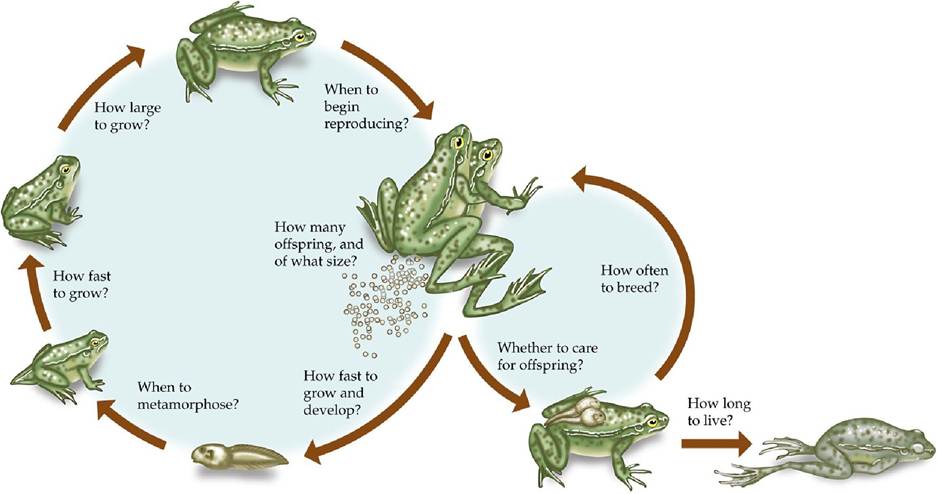
FIGURE 7.3 Life History Strategy The timing and nature of life history events shapes the overall life cycle of an organism. Although life history options are presented here as questions, the
life history strategy is determined by effects of natural selection, not the choices of the individual organism. View larger image
The life history strategy is shaped by the way the organism divides its energy and resources between growth, reproduction, and survival, and the associated trade-offs with the allocation patterns. Within a species, individuals often differ in how they divide their energy and resources among these activities. Such differences affect the ecological success of a species and may result from genetic variation, from differences in environmental conditions, or from a combination of both.
Genetic Differences
Some life history variation within species is determined genetically. Genetically influenced traits can often be recognized as those that are more similar within families than between them.
Again, these kinds of traits are familiar in humans: for example, siblings are often similar in appearance and reach similar adult heights and weights. The same is true in other organisms. For example, in annual bluegrass (Poa annua), life history traits such as age at first reproduction, growth rate, and number of flowers produced are similar among sibling plants (Law et al. 1977). As with any other trait, heritable variation in life history traits is the raw material on which natural selection acts. Selection favors individuals whose life history traits result in their having a better chance of surviving and reproducing than do individuals with other life history traits.Much of life history analysis is concerned with explaining how and why life history patterns have evolved to their present states. Life histories are believed to be adapted to maximize fitness (the genetic contribution of an organism's descendants to future generations, determined both by the reproductive rate of the parent and the survival rates of both parent and offspring). However, no organism has a perfect life history—that is, one that results in the unlimited production of descendants. Instead, all organisms face constraints that prevent the evolution of a perfect life history. As we'll see in Concept 7.3, these constraints often involve ecological trade-offs in which an increase in the performance of one function (such as reproduction) can reduce the performance of another (such as growth or survival). Thus, although life histories often serve organisms well in the environments in which they have evolved, they are optimal only in the sense of maximizing fitness subject to constraints.
Environmental Differences
A single genotype may produce different phenotypes under different environmental conditions, a phenomenon known as phenotypic plasticity (see the Climate Change Connection in Chapter 6). Almost every trait shows some degree of plasticity, and life history traits are no exception.
For example, most plants and animals grow at different rates depending on temperature. They do so because development typically speeds up as the temperature rises, then slows down again due to heat stress as the temperature approaches the organism's upper lethal temperature.Changes in life history traits often translate into changes in adult morphology. Slower growth under cooler conditions, for example, may lead to a smaller adult size or to differences in adult shape. Callaway et al. (1994) showed that ponderosa pine (Pinus ponderosa) trees grown in cool, moist climates allocate more biomass to leaf growth relative to sapwood production than do those in warmer desert climates (“sapwood” refers to newly formed layers of wood that function in water transport). Allocation describes the relative amounts of energy or resources that an organism devotes to different functions. The result of allocation differences in ponderosa pines is that trees grown in different environments differ in adult shape and size. Desert trees are shorter and squatter, with fewer branches and leaves (FIGURE 7.4). As a result of having fewer leaves, they also lose less water and have lower photosynthetic rates per unit of ground area.
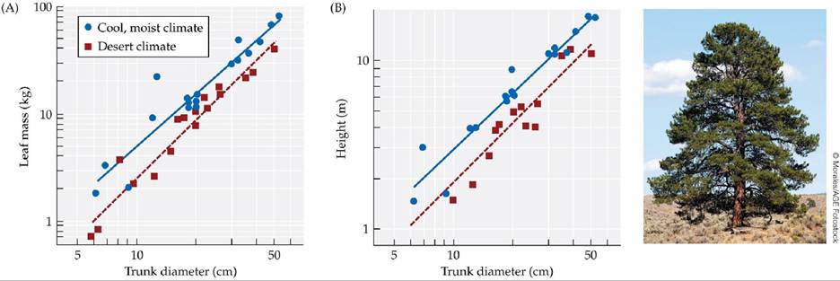
FIGURE 7.4 Plasticity of Growth Form in Ponderosa Pines (A) Ponderosa pine trees (Pinus ponderosa) in cool, moist climates allocate more resources to leaf production than do trees in desert climates. (B) Desert trees are shorter than those grown in cooler climates, but for a given height, they have thicker trunks.
Use the solid (regression) line in (B) to estimate the trunk diameter of a tree that is 5 m tall and grows in a cool, moist climate versus the trunk diameter of a tree of the same height that grows in a desert climate.
(After R. M. Callaway et al. 1994. Ecology 75: 1474-1481.) View larger image
Phenotypic plasticity that responds to temperature variation often produces a continuous range of sizes. In other types of phenotypic plasticity, a single genotype produces discrete types, or morphs, with few or no intermediate forms.
For example, populations of spadefoot toad (Spea multiplicata) tadpoles in Arizona ponds contain two morphs: omnivore morphs, which feed on detritus and algae, and larger carnivore morphs, which feed on fairy shrimp and on other tadpoles (FIGURE 7.5). The differing body shapes of omnivores and carnivores result from differences in the relative growth rates of different body parts: carnivores have bigger mouths and stronger jaw muscles because of accelerated growth in those areas. Pfennig (1992) showed that omnivore tadpoles can turn into carnivores when fed on shrimp and tadpoles, and field studies show that the proportion of omnivore and carnivore morphs is affected by food supply. Carnivore tadpoles grow faster and are more likely to metamorphose before the ponds where they live dry up. As a result the rapidly growing carnivores are favored in ephemeral ponds. The more slowly growing omnivores are favored in ponds that persist longer, because they metamorphose in better condition and thus have better chances of survival as juvenile toads.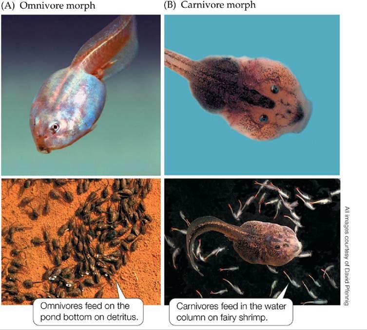
FIGURE 7.5 Phenotypic Plasticity in Spadefoot Toad Tadpoles Spadefoot toad (Spea multiplicata) tadpoles can develop into small-headed omnivores (A) or large-headed carnivores (B), depending on the food they consume early in development. Later in development, omnivores and carnivores feed on different food sources that are located in different portions of their habitat. View larger image
Examples of phenotypic plasticity such as the omnivore and carnivore morphs of the spadefoot toad may suggest situations where phenotypic plasticity is adaptive —that the ability to produce different phenotypes in response to changing environmental conditions increases the fitness of individuals. While that is often the case, adaptation must be demonstrated rather than assumed. For example, it may be adaptive for ponderosa pines to be stockier and have fewer leaves in hot, dry climates because these features can help reduce water loss.
However, adaptation would have to be documented by measuring and comparing the survival and reproductive rates of stockier and taller trees in the desert environment. In some instances, phenotypic plasticity may be a simple physiological response, not an adaptive response shaped by natural selection. For example, as mentioned above, growth rate typically increases with temperature up to a point. This may occur because chemical reactions are slower at lower temperatures, and thus metabolism and growth are necessarily slower.Climate Change Connection
Climate Change and the Timing of Seasonal Activities
The timing of seasonal life history activities can be of critical importance. For example, a bird that migrates north too early in the spring may starve if no food is available, while a plant that flowers when its pollinators are not present may fail to reproduce. As described in Concept 4.2, the timing of such seasonal events is affected by changing day length (photoperiod) and sometimes by other environmental cues such as temperature that also vary over the course of a year. As the climate has changed in recent decades, have species adjusted the times when they perform key seasonal activities?
Long-term data sets show that many species are initiating spring activities earlier than they once did in response to climate change. For example, as the climate warms, leaf production in plants, egg laying in birds, emergence from dormancy in insects, and arrival of migratory animals often occur earlier today than they did in the 1960s and 1970s.
In some cases, however, shifts in the timing of seasonal activities have not kept pace with climate change. One example involves seasonal change in fur coloration of the snowshoe hare (Lepus americanus). As winter approaches, the coat color of snowshoe hares changes from brown to white, providing camouflage against snow; the reverse coat-color change occurs in spring. As the climate has warmed, the length of time that the ground is covered by snow has decreased because snowfall now begins later in autumn and snowmelt occurs earlier in spring.
If the timing of the fall coat-color change in snowshoe hares had kept pace with the delay in when snowfall begins, we would expect that snowshoe hares would molt to white later in the fall than they once did. Instead, however, the date and rate of the fall molt has not changed (Mills et al. 2013). As a result, the number of days in which a “camouflage mismatch” occurs has increased, making the hares easier for visually hunting predators to spot (FIGURE 7.6) and leading to increased mortality rates (Zimova et al. 2016). Mismatches in the timing of seasonal activities have also been found in caribou (Rangifer tarandus) and snow geese (Chen caerulescens): although the plants their young require for food are producing leaves earlier in the spring, neither species has adjusted the timing of reproduction. This has caused a decline in the reproductive success of both species because their young are not getting enough to eat.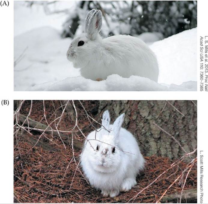
FIGURE 7.6 Camouflage Mismatch in Snowshoe Hares (A) Historically, snowshoe hares changed their color from brown to white at a time of year that matched the onset of snowfall, causing them to be well-camouflaged all winter. (B) With climate warming, snowfall now begins later in the year. However, the date of the fall coat-color change has remained the same, causing an increase in the number of days that snowshoe hares experience a camouflage mismatch. Vi6w larg6r imag6