Populations grow geometrically when reproduction occurs at regular time intervals
Some species, such as cicadas and annual plants, reproduce in synchrony at regular time intervals. These regular time intervals are called discrete time periods. Geometric growth occurs when a population with synchronous reproduction changes in size by a constant proportion from one discrete time period to the next.
The fact that the population grows by a constant proportion means that the number of individuals added to the population becomes larger with each time period (births > deaths). As a result, the population grows larger by ever-increasing amounts. When plotted on a graph, this growth pattern forms a J-shaped set of points, with each point representing the resulting population size after each time period (FIGURE 11.4A).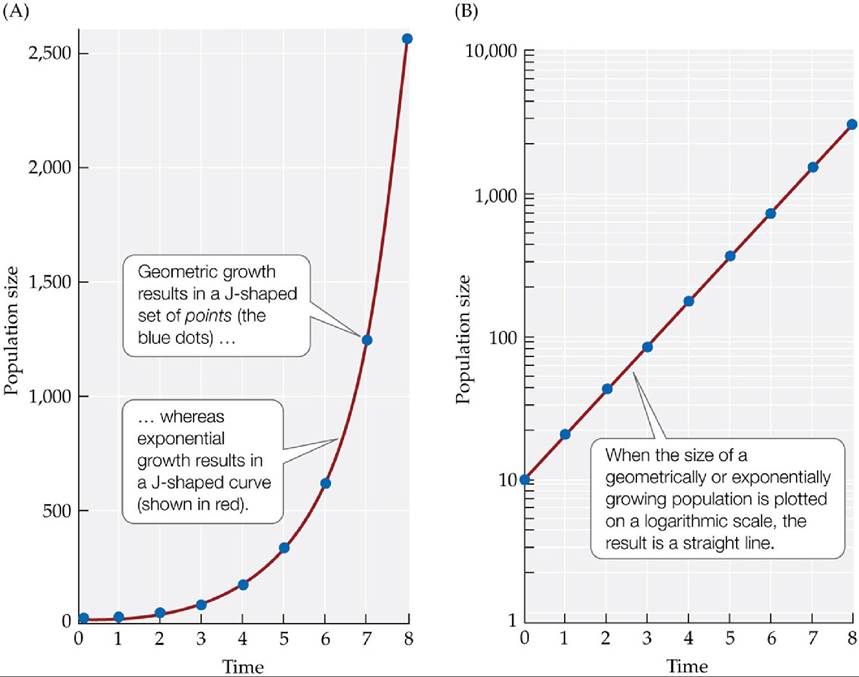
FIGURE 11.4 GeometricandExponentialGrowth (A) The blue dots plot the size of a geometrically growing population that begins with 10 individuals and doubles in each discrete time period (i.e., No = 10 and λ = 2). The red curve plots exponential growth in a comparable population that reproduces continuously, also beginning with 10 individuals and having a growth rate of r = ln(2) = 0.69. (B) When the population sizes represented by the blue circles and the red curve in (A) are plotted on a logarithmic scale, the result is a straight line. View larger image
Mathematically, we can describe geometric growth as

(11.1)
where Nt is the population size after t generations or, equivalently, after t discrete time periods (e.g., t years if there is one generation per year), and λ is a constant whose value is determined by the per capita (or per individual) birth rate (b =
B/N) minus the per capita death rate (d = D/N) over discrete time periods.
In Equation 11.1, λ serves as a multiplier that allows us to predict the size of the population in the next time period. We'll refer to λ as the geometric population growth rate; λ is also known as the (per capita) finite rate of increase. We use this terminology by convention, but it can be confusing: we can see from Equation 11.1 that when the population “growth” rate λ is between 0 and 1, the population does not grow, but rather decreases in size over time.Geometric growth can also be represented by a second equation,
(11.2)
where N0 is the initial population size (i.e., the population size at time = 0).
The two equations for geometric growth (Equations 11.1 and 11.2) are equivalent in that each can be derived from the other. Which one we use depends on what we are interested in. If we want to predict the population size in the next time period and we know λ and the current population size, either equation can be used. If we know the population size in both the current and previous time periods, we can rearrange Equation 11.1 by dividing Nt+1 by Nt to get an estimate of λ. Finally, we can use Equation 11.2 to predict the size of the population after any number of discrete time periods. If λ = 2, for example, then after 12 time periods, a population that begins with N0 = 10 individuals will have N12 = 212N0 individuals, which (as we can determine by using a calculator with a yx function) equals 4,096 ? 10, or 40,960.
Populations grow exponentially when reproduction occurs continuously
In contrast to the pattern described in the previous section, individuals in many species (including humans) do not reproduce in synchrony at discrete time periods; instead, they reproduce continuously over time. Exponential growth occurs when population size changes by a constant proportion at each instant in time (see the red curve in Figure 11.4A, representing continuous growth).
Mathematically, exponential growth can be described by the following two equations: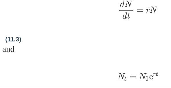
(11.4)
where Nt is the population size at each instant in time, t.
In Equation 11.3, dN/dt represents the rate of change in population size at each instant in time; we see from the equation that dN/dt equals a constant rate (r; instantaneous birth rate (b) - instantaneous death rate (d)) multiplied by the current population size, N. Thus, the multiplier r provides a measure of how rapidly a population can grow; r is called the exponential growth rate or the (per capita) intrinsic rate of increase.
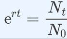
As we did for Equation 11.2, we can use Equation 11.4 to predict the size of an exponentially growing population at any time t, provided we have an estimate for r and know N0, the initial population size. The “e” in Equation 11.4 is a constant, approximately equal to 2.718 [“e” is the base of the natural logarithm, ln(x)]. We can calculate ert using the function ex, which can be found on many calculators.
When plotted on a graph, the exponential growth pattern forms a curve that, like the geometric growth pattern, is J-shaped. Exponential growth and geometric growth are similar in that we can draw an exponential growth curve through the discrete points of a population that grows geometrically (see Figure 11.4A). Because exponential and geometric growth curves overlap, both types of growth are sometimes lumped together for simplicity and referred to as exponential growth.
Geometric and exponential growth curves overlap because Equations 11.2 and 11.4 are similar in form, except that λ in Equation 11.2 is replaced by er in Equation 11.4. Thus, if we want to compare the results of discrete time and continuous time growth models, we can calculate λ from r, or vice versa:
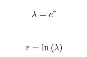
where ln(λ) is the natural logarithm of λ, or loge(λ).
For example, if λ = 2 (as in Figure 11.4A), an equivalent value for r would be r = ln(2), which is approximately 0.69. FIGURE 11.4B illustrates a simple way to determine whether a population really is growing exponentially: plot the natural logarithm of population size versus time, and if the result is a straight line, the population is increasing exponentially.Finally, look again at Equations 11.1 and 11.3. In Equation 11.1, which value of λ will ensure that the population does not change in size from one time period to
the next? Similarly, in Equation 11.3, which value of r causes the population to remain fixed in size? The answers are λ = 1 (because then Nt+1 = Nt) and r = 0 (because then the rate at which the population size changes is 0). When λ < 1 (or r < 0), the population will decline to extinction, whereas when λ > 1 (or r > 0), the population will increase geometrically (or exponentially) to form a J-shaped curve (FIGURE 11.5).
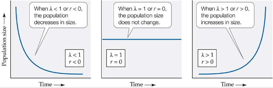
FIGURE 11.5 How Population Growth Rates Affect Population Size Depending on the value of λ or r, a population with an exponential growth pattern will decrease in size, remain the same size, or increase in size. View larger image
How can we estimate a population's growth rate (r or λ)? In one approach, Equation 11.4 is used to estimate the growth rate r at different points in time, as you can explore for the human population in ANALYZING DATA 11.1. There are a variety of other methods as well (see Caswell 2001), including estimating r (or λ) from life table data, as we will see in Concept 11.4.
Z v∙
ANALYZING DATA 11.1
How Has the Growth of the Human Population Changed over Time?
Ecologists often use estimates of λ or r to determine how rapidly a
population is growing (or declining) at various points in time. For a population that is growing exponentially, we can calculate such estimates by rearranging Equation 11.4 to read
where N0 is the population size at the beginning of a time period, t is the length of the time period, and Nt is the population size at the end of the period.
If we know t, N0, and Nt, we can then estimate r: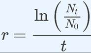
In this exercise, we'll use this technique and the data in the table to examine the growth rate of the world's human population at different points in time.
1. Calculate the exponential growth rates for the years shown in the table and graph your results. For example, from year 1 to year 400, the length of the time period, t, is t = 400 - 1 = 399, and we find that r = [ln(190 million/170 million)]∕399 = 0.1112/399 = 0.00028.
| Year (C.E.) | Population size | Exponential growth rate (r) |
| 1 | 170 million | 0.00028 |
| 400 | 190 million | ? |
| 800 | 220 million | ? |
| 1200 | 360 million | ? |
| 1550 | 500 million | ? |
| 1804 | 1 billion | ? |
| 1927 | 2 billion | ? |
| 1960 | 3 billion | ? |
| 1999 | 6 billion | ? |
| 2010 | 6.87 billion | ? |
| 2016 | 7.35 billion | ? |
| 2019 | 7.7 billion | (N/A) |
2. If the human population continued to grow at the rate you calculated for 2016, how large would the population be in 2066?
3. What assumptions did you make in answering Question 2? Based on results for Question 1, is it likely that the human population will reach the size that you calculated for 2066? Explain.
We can also use r to determine the doubling time (td) of a population, which is the number of years it will take the population to double in size. As interested readers can confirm (by solving Equation 11.4 for the time it takes a population to increase from its initial size, N0, to twice that size, 2N0), doubling times can be estimated as 
(11.5)
where r is the exponential growth rate.