BROADENING THE SCOPE

24.5.1 Extended Income, Consumption and Indirect Taxes

Although disposable income is the most-used indicator of living standard, it is widely recognized that economic well-being is a multidimensional concept (see Chapter 2).

In European countries, in-kind benefits, such as services related to child and elderly care, education, health, and public housing, represent about half of welfare state support and contribute to reducing the inequality otherwise observed in the cash income distri­bution. The economic value of public in-kind benefits can be imputed at individual and household levels on the basis of per capita spending, considering the average cost of pub­lic services (such as providing care and education services), the gain from paying below- market rent or no rent at all for public housing, or the risk-related insurance value approach that considers public health care services equivalent to purchasing an insurance policy with the same cost for individuals who have the same sociodemographic charac­teristics.

A more comprehensive measure of individual command over resources should include the income value of home ownership as well. This is because the consumption opportunities of homeowners (or individuals living in reduced or free rent housing) differ from those of other individuals due to the imputed rent that represents what they would pay if they lived in accommodation rented at market prices. The inclusion of imputed rent in microsimulation models is becoming more common due to the refinement of different methods for deriving a measure of imputed rent (Frick et al., 2010) and also a renewed interest in property taxation. From a cross-country perspective, Figari et al. (2012b) analyze the extent to which including imputed rent in taxable income affects the short-run distribution of income and work incentives, showing a small inequality­reducing effect together with a nontrivial increase in tax revenue. This offers the opportunity to shift the fiscal burden away from labor and to increase the incentive for low-income individuals to work.

Indirect taxes typically represent around 30% of government revenue. With only a few exceptions, household income surveys providing input data for microsimulation models do not include detailed information on expenditures either, preventing micro­level analysis of the combined effect of direct and indirect taxation. The solution usually adopted to overcome this data limitation is to impute information on expenditures into income surveys (Sutherland et al., 2002).

Most microsimulation models that include the simulation of indirect taxes rely on the assumption of fixed producer prices, with indirect taxes fully passed to the final price paid by the consumer. To relax such an assumption one should go beyond a partial equilibrium framework and link the microsimulation models to macro models (see Section 24.3.4) in order to consider the producer and consumer responses to specific reforms or economy­wide shocks.

The inclusion of indirect taxes also raises the question of how to measure their inci­dence. Table 24.1 shows the incidence of indirect tax payments for three European

Table 24.1 Incidence of indirect tax payments

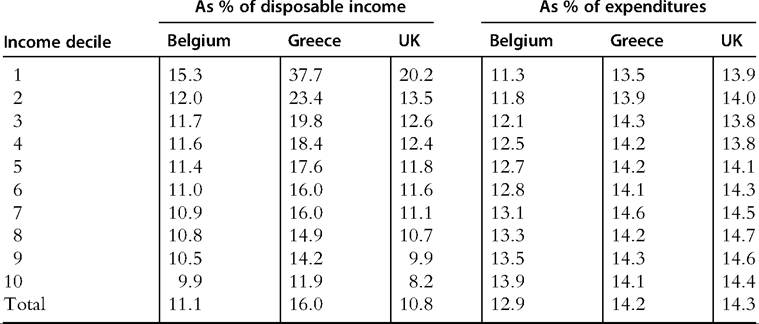
Notes: Decile groups are formed by ranking individuals according to equivalized household disposable income, using the modified OECD equivalence scale.

Source: Figari and Paulus (2013), based on EUROMOD.

countries expressed as a percentage of disposable income and as a percentage of expen­diture, by decile of equivalized disposable income. In the first case (see the left panel of Table 24.1), the regressivity of indirect tax payments is clear: poorer individuals pay a larger proportion of their income in indirect taxes compared to richer individuals, mainly due to a larger propensity to consume or even dissaving reflected by average expenditures exceeding incomes for the individuals at the bottom of the income distribution (Decoster et al., 2010). However, survey data might suffer from measurement error, in particular from income underrecording (Brewer and O’Dea, 2012), which could give a misleading snapshot of the income-consumption pattern at the bottom of the income distribution. In thesecond case (i.e., the rightpanel of Table 24.1), indirect tax payments are progressive, and poorer individuals pay a slightly smaller proportion of their total expenditure in VAT and excises compared to richer individuals.

The potential of microsimulation models that are capable of simulating direct and indirect taxes within the same framework is reinforced by the renewed interest in the tax shift from direct to indirect taxation in order to enhance the efficiency of the tax system (Decoster and Van Camp, 2001; Decoster et al., 2010). In particular, microsimulation models have been used to assess the distributional consequences of a “fiscal devaluation,” a revenue-neutral shift from payroll taxes toward value-added taxes that might induce a reduction in labor costs, an increase in net exports, and a compression ofimports, with an overall improvement in the trade balance (de Mooij and Keen, 2013; European Commission, 2013).

Two general considerations arise from the use of microsimulation models for the anal­ysis of the redistributive effects of indirect taxes. On the one hand, the actual degree of regressivity of indirect taxes might be less than that observed if surveys tend to underre­port income more than consumption at the bottom of the income distribution (Brewer and O’Dea, 2012; Meyer and Sullivan, 2011). On the other hand, a more systematic use of simulated income values, as generated by a microsimulation model rather than as observed in the data, can help in solving the underreporting of income values, closing the gap between reported income and consumption and providing a more robust indi­cator of living standards for those with a low level of resources.

24.5.2 Dynamic Microsimulation and Lifetime Redistribution

The importance of investigating the “long-range character” of public policies was already highlighted by Guy Orcutt in the 1950s (Orcutt, 1957) and pioneered through his work in the 1970s on DYNASIM, a dynamic microsimulation model of the US designed to analyze the long-term consequences of retirement and aging issues (Orcutt et al., 1976). A number of reviews survey the existing dynamic microsimulation models, the method­ological challenges, and the types of uses, providing an overall picture of the evolution of the state of play and future research directions for interested readers (Gupta and Harding, 2007; Harding, 1993, 1996b; Harding and Gupta, 2007; Li and O’Donoghoue, 2013; Mitton et al., 2000).

Dynamic microsimulation models extend the time frame of the analysis in order to address the long-term distributional consequences of policy changes, widening the per­spective of the effects of the policies to encompass the individual lifetime and addressing questions about intrapersonal redistribution over the lifecycle (Harding, 1993). Dynamic microsimulation models typically aim to capture two main factors that shape the income distribution in a long-term perspective. First, they cover the changing structure of the population due to evolving individual and household characteristics (e.g., age, education, household composition) and life events (e.g., marriage, household formation, birth, migration). Second, they capture the interaction of market mechanisms (e.g., labor mar­ket participation, earnings levels) and the tax-benefit system with such characteristics in each point in time.

In particular, they are useful tools to analyze: (i) the performance oflong-term policies such as pensions and other social insurance programs such as health and long-term care, (ii) the consequences of different demographic scenarios, (iii) the evolution of intertem­poral processes and behaviors such as wealth accumulation and intergenerational transfers, and (iv) the geographical trend of social and economic activities if dynamic microsimulation models are supplemented with spatial information (Bourguignon and Bussolo, 2013; Li and O’Donoghoue, 2013).

The methodological challenges behind a microsimulation model depend on the scope of the events taken into account and the methodology used to age the population of interest through the period of analysis. The aging process can be either static or dynamic. With the static aging method, the individual observations are reweighted to match exist­ing or hypothetical projections of variables of interest. The approach is relatively straight­forward, but it can become unsatisfactory if the number of variables to be considered simultaneously is large or if one is interested in following individual transitions from one point in time to the next (see also Section 24.3.5.1). The dynamic aging method builds up a synthetic longitudinal dataset by simulating individual transition probabilities conditioned on past history and cohort constraints that take into account the evolution of the sociodemographic characteristics of interest through the time horizon of the analysis (Klevmarken, 2008). The major source of information for the estimation of the dynamic processes is derived from longitudinal data available in most developed countries, although often the duration of the panel is not long enough to observe transitions for large samples of individuals, the main exceptions being the long panel data available in Australia, Germany, the UK, and the US. Transitions can be estimated through reduced form models that incorporate deterministic and stochastic components, or they can be simulated, taking into account behavioral reactions of individuals to other changes that occurred at the same time, based on individual preferences estimated through structural models that take into account the endogeneity of some individual transition probabilities (see Section 24.3.3).

The aging of individual and household characteristics can be implemented as a dis­crete or continuous process. The former is usually built around yearly time intervals; it is more straightforward but implies that some simulated events might not respect the real sequence. The latter is based on survival functions that consider the joint hazard of occurrence of the simulated events.

In principle, dynamic microsimulation models allow for analysis that is more in line with the theoretical arguments in favor of a lifetime approach to the analysis of the redis­tributive effects of tax-benefit systems, as developed in the welfare economics literature (Creedy, 1999a). Nelissen (1998) is one of the few examples where the annual and lifetime redistributive effects of the social security system (here for the Netherlands) are analyzed simultaneously, making use of the same microsimulation model that guar­antees comparable simulations of the tax-benefit system in place over a long period of time. In line with other research (e.g., Harding, 1993), Nelissen (1998) finds that the lifetime redistributive effect is considerably smaller than the annual incidence, with important policy implications due to the different incidence of various pension schemes on different generations.

Due to the complexity of the aging process, early dynamic microsimulation models tended not to address the long term implications of policy and policy change on income distribution as a whole (i.e., population-based models) but rather focused on specific cohorts of the population (cohort models). Nowadays such a distinction is less significant due to the improvements in the modeling set up as well as major improvements in avail­able computing power. However, despite the improvements in dynamic microsimula­tion modeling, such models are often perceived as black boxes, making it difficult to understand and appreciate their properties. In particular, the lack of good economic the­ory and sound econometric inference methods are thought to contribute to a sceptical view of these models by the economics profession (Klevmarken, 2008).

Two particular research developments characterize the dynamic microsimulation field. First, this is an area where international collaborations are emerging in an attempt to reduce the efforts needed to build very complex models. The Life-Cycle Income Analysis Model (LIAM) stands out as a viable option to provide a general framework for the construction of new dynamic microsimulation models (O’Donoghue et al., 2009) and to be linked to EUROMOD (and other modular-based microsimulation models) in order to exploit the existing parameterization of tax-benefit systems for the European countries (Liegeois and Dekkers, 2014). Second, most dynamic microsimula­tion models do not include macro feedback effects and do not have market clearing mechanisms that would require ambitious links to macro models (Bourguignon and Bussolo, 2013). However, due to the number and complexity of the interactions between many social and economic variables involved in the modeling, the integration between dynamic micro and macro models could introduce too much uncertainty in the results to make them useful in a policy context (Li and O’Donoghoue, 2013).

24.5.3 Crossing Boundaries: Subnational and Supranational Modeling

The natural territorial scope for a microsimulation model is a country or nation. This is because in most countries some or all of the tax-benefit system is legislated and admin­istered nationally; the micro-data used as an input dataset are representative at the national level; the other data used to update, adjust, and validate the model are usually made avail­able at national level; and the economy and society are usually assumed to exist and oper­ate at this level. However, in some countries, policies can vary across regions, sometimes following from (or accompanied by) major differences in politics, history, and economic and social characteristics. In some cases, the data that are especially suitable as the basis for microsimulation modeling are only available for one region. For these reasons, models may exist for single regions, or national models may be able to capture regional differ­ences in policy. Examples of regional or subnational models include Decancq et al. (2012) for Flanders (Belgium) and Azzolini et al. (2014) for Trentino (Italy); both are based on the EUROMOD framework, and the latter exploits a rich dataset that combines

administrative and survey data. Examples of national modeling exercises that capture extensive regional differences in policies include Canto et al. (2014) for Spain.

If the micro-data are representative of each region, then the national model can oper­ate as a federation of regional models, also capturing any national policy competencies. As well as simulating the appropriate policy rules regardless of location (many models for countries with regional policy variation simply opt to simulate policies from a single “representative” region), these federal models can identify the implied flows of resources (redistribution) between regions as well as within them, given budget constraints at either national or regional levels. In the US, the most comprehensive in terms of policy coverage is the long-standing microsimulation model, TRIM3, which simulates welfare programs, as well as taxes and regional variation in programs, making use of a common national input dataset: the Current Population Survey (CPS) Annual Social and Economic Supplement (ASEC). ⁰ See, for example, Wheaton et al. (2011) who compare the effects of policies on poverty across three U.S. states. For Canada, the microsimula­tion model SPSD/M has been linked to a regional input-output model in order to cap­ture some of the indirect effects of national or provincial tax-benefit policy changes at the provincial level (Cameron and Ezzeddin, 2000).

In the European Union, policies in the 28 member states vary in structure and pur­pose to a much greater degree than they do across US states. Although the EU-SILC data is output-harmonized by Eurostat, it is far from ideal as an input database for a micro­simulation model (Figari et al., 2007), and significant amounts of nationally specific adjustments are needed to provide the input data for EUROMOD, the only EU-wide model (see Box 24.1). Indeed, although the supranational administration of the EU has no relevant policy-making powers (at the time of writing), analysis that considers the EU (or the eurozone) as a whole is highly relevant to approaching the design of tax-benefit policy measures to encourage economic stabilization and social cohesion. Analogously to regionalized national models, EUROMOD is able to draw out the implications of potential EU-level policy reforms for both between- and within-country redistribution (Levy et al., 2013), policy harmonization, and stabilization (Bargain et al., 2013a), as well as for the EU income distribution.

At the other extreme, microsimulation methods have been used to estimate income distribution and other indicators for small areas. This relies on spatial microsimulation techniques (Tanton and Edwards, 2013) or, more commonly, reweighting national or regional micro-data so that key characteristics match those from census data for the small area (Tanton et al., 2011). In the developed world, policymakers generally use these models to predict the demand for services such as care facilities (for example, Lymer et al. (2009) for Australia and Wu and Birkin (2013) for the UK). In circumstances where the census data provide a good indication of income levels, such as in Australia, they have

also been used to provide small area estimates of income distribution and its components (Tanton et al., 2009). Linkage of the census with household budget survey data in the UK has been used to estimate the small area effects of an increase in VAT (Anderson et al., 2014). A similar method known as “poverty mapping” has been applied to developing countries by Elbers et al. (2003), using household budget surveys and census micro-data in order to monitor the geographic concentration of poverty and to evaluate geographic targeting of the poor as a way of rebalancing growing welfare disparities between geographic areas. For the use of the model for Vietnam, see Lanjouw et al. (2013).

24.6.