Consumption and saving
Consumption is the most important single element in aggregate demand, accounting for almost half of gross final expenditure (GFE), so that its accurate estimation is essential to the management of the economy.
J. M. Keynes related consumption to current disposable income, and for many years this was widely accepted. However, in the 1950s evidence began to appear of a discrepancy between the consumption function estimated from long-run time-series data, and the much flatter consumption function estimated from short-run time-series and cross-section data. The Keynesian consumption function could not resolve this discrepancy, and it was this, together with the need for more accurate forecasts of consumption, that led to the development of the Permanent Income and Life Cycle Hypotheses. In this chapter the Keynesian and alternative theories of consumption are considered in detail, their predictions are compared with actual fact, and their different implications for policy analysis are noted. We also look carefully at the mirror image of consumption, namely the savings ratio.Consumption
The Keynesian consumption function
The consumption function - the relationship between consumer expenditure and income - is probably the most widely researched relationship in macroeconomics. The impetus to this research was given by Keynes’s initial conceptual breakthrough in The General Theory of Employment, Interest and Money (Keynes 1936). In the Keynesian view of the economic system, both output and employment are determined by the level of aggregate demand. Consumer spending is by far the largest element in aggregate demand. Typically it accounts for between half and two-thirds of total final expenditure, so it is essential that the factors influencing consumer spending be identified in order that it may be forecast accurately. This forecast for consumer spending can then be added to forecasts for the other elements of aggregate demand, namely investment, government spending and net exports (exports minus imports), to derive an overall forecast for total aggregate demand.
Policy-makers can then decide whether this projected level of demand is appropriate for the economy and, if not, what corrective fiscal or monetary action should be taken.The central position of the consumption function in Keynesian economics has therefore led to many attempts to estimate an equation that would indeed predict consumer expenditure. Unfortunately, most of the early Keynesian types of equation failed to explain some of the more interesting features of aggregate consumer behaviour. Alternative theories were therefore developed in the 1950s and 1960s which, it was claimed, fitted the facts rather better than the simple Keynesian view of consumption.
The development of these new theories, and the relative economic stability of the 1950s and 1960s, led economists to believe (over-optimistically as it turned out) that consumer spending was probably one of the best-understood and best-forecast variables in economics. We see from Table 16.1, however, that there was a sharp fall in the proportion of personal disposable income consumed (the average propensity to consume, a.p.c.) in the early and late 1970s, early 1980s and early 1990s and a sharp rise in the late 1980s, the mid 1990s and recently which were not always predicted by the existing equations. These changes in the a.p.c. were reflected in the sharp rise or fall in the savings ratio, and we return to changes in the savings ratio, later in the chapter.
In the General Theory, Keynes argued that ‘The fundamental psychological law... is that men are disposed, as a rule and on the average, to increase their consumption as their income increases, but not by as much as the increase in their income’ (Keynes 1936, p. 96). From this statement can be derived the Keynesian consumption function1 which is usually expressed in the following way:
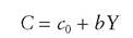
where C = consumer expenditure;
c0 = a constant;
b = the marginal propensity to consume (m.p.c.), which is the amount consumed out of the last pound of income received; and
Y = National Income.
The Keynesian view is that when income rises, consumption rises, but by less than income, which implies that b, the m.p.c., is less than 1. Keynes also argued that ‘it is also obvious that a higher absolute level of income will tend, as a rule, to widen the gap between income and consumption’ (Keynes 1936, p. 97). This is usually taken to mean that he thought that the proportion of income consumed, C/Y (i.e. a.p.c.), will tend to fall as income increases. In fact, the positive constant c0 in the above equation ensures that this will happen, since
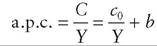
and this will decrease as Y increases if, and only if, c0 is positive. This also implies, of course, that the a.p.c. is greater than the m.p.c. by an amount c0/Y.
Drawing the consumption function as a straight line, as in Fig. 16.1, means that we are assuming that the m.p.c., b, is a constant, as it is the slope of the consumption function. The a.p.c. is found, for any level of income, by measuring the slope of the radian from the origin to the appropriate point on the consumption function. For example, if income is Y1, then consumption would be C1, and the a.p.c. would be C1∕Y1, which is the tangent of the angle α. It can be seen that as Y increases, the slope of the radian from the origin to the consumption function falls, which
Table 16.1 UK household income, consumption and savings ratio, 1970-2009 (£m at 2006 prices).
| 1 Disposable income | 2 Consumption | 3* Average propensity to consume (a.p.c.) | 4 Change in income | 5 Change in consumption | 6* Marginal propensity to consume (m.p.c.) | 7 Household savings ratio (%) | |
| 1970 | bgcolor=white>320,056297,462 | 0.93 | 6.6 | ||||
| 1971 | 323,930 | 307,172 | 0.95 | 3,874 | 9,710 | 2.51 | 5.0 |
| 1972 | 350,987 | 326,989 | 0.93 | 27,057 | 19,817 | 0.73 | 7.3 |
| 1973 | 373,092 | 344,928 | 0.92 | 22,105 | 17,939 | 0.81 | 8.2 |
| 1974 | 369,501 | 339,885 | 0.92 | -3,591 | -5,043 | 1.40 | 8.4 |
| 1975 | 372,138 | 338,945 | 0.91 | 2,637 | -940 | -0.36 | 9.2 |
| 1976 | 370,056 | 340,035 | 0.92 | -2,082 | 1,090 | -0.52 | 8.7 |
| 1977 | 362,096 | 338,535 | 0.93 | -7,960 | -1,500 | 0.19 | 7.6 |
| 1978 | 385,500 | 356,311 | 0.92 | 26,404 | 17,776 | 0.67 | 9.4 |
| 1979 | 411,329 | 372,864 | 0.91 | 22,829 | 16,553 | 0.73 | 10.9 |
| 1980 | 418,940 | 372,589 | 0.89 | 7,611 | -275 | -0.04 | 12.3 |
| 1981 | 417,974 | 372,726 | 0.89 | -966 | 137 | -0.14 | 12.0 |
| 1982 | 418,508 | 376,298 | 0.90 | 534 | 3,572 | 6.69 | 10.8 |
| 1983 | 427,443 | 392,035 | 0.92 | 8,935 | 15,737 | 1.76 | 9.0 |
| 1984 | 443,605 | 400,798 | 0.90 | 16,162 | 8,763 | 0.54 | 10.2 |
| 1985 | 459,081 | 415,952 | 0.91 | 15,476 | 15,154 | 0.98 | 9.7 |
| 1986 | 478,649 | 443,391 | 0.93 | 19,568 | 27,539 | 1.41 | 8.1 |
| 1987 | 486,579 | 467,794 | 0.96 | 7,930 | 24,303 | 3.06 | 5.4 |
| 1988 | 513,846 | 503,656 | 0.98 | 27,267 | 35,862 | 1.32 | 3.9 |
| 1989 | 538,605 | 521,294 | 0.97 | 24,759 | 17,638 | 0.71 | 5.7 |
| 1990 | 563,135 | 525,408 | 0.93 | 24,530 | 4,114 | 0.17 | 8.1 |
| 1991 | 574,060 | 516,933 | 0.90 | 10,925 | -8,475 | -0.78 | 10.3 |
| 1992 | 589,636 | 519,291 | 0.88 | 15,576 | 2,358 | 0.15 | 11.7 |
| 1993 | 607,421 | 532,860 | 0.88 | 17,785 | 13,569 | 0.63 | 10.8 |
| 1994 | 615,909 | 547,735 | 0.89 | 8,488 | 14,875 | 1.17 | 9.3 |
| 1995 | 631,068 | 557,865 | 0.98 | 16,059 | 10,130 | 0.81 | 10.3 |
| 1996 | 651,252 | 589,437 | 0.89 | 19,284 | 22,572 | 1.78 | 9.4 |
| 1997 | 678,717 | 602,610 | 0.99 | 27,465 | 22,173 | 0.81 | 9.6 |
| 1998 | 692,847 | 627,710 | 0.91 | 14,130 | 25,100 | 1.78 | 7.4 |
| 1999 | 712,729 | 661,427 | 0.93 | 19,882 | 33,717 | 1.70 | 5.2 |
| 2000 | 742,664 | 691,461 | 0.93 | 29,935 | 30,034 | 1.00 | 4.7 |
| 2001 | 775,651 | 713,535 | 0.92 | 32,987 | 22,074 | 0.67 | 6.0 |
| 2002 | 791,488 | 739,832 | 0.93 | 15,837 | 26,297 | 1.66 | 4.8 |
| 2003 | 815,076 | 762,772 | 0.94 | 23,588 | 22,940 | bgcolor=white>0.975.1 | |
| 2004 | 823,672 | 787,523 | 0.96 | 8,596 | 24,751 | 2.88 | 3.7 |
| 2005 | 840,358 | 805,273 | 0.96 | 16,686 | 17,750 | 1.06 | 3.9 |
| 2006 | 853,095 | 819,610 | 0.96 | 12,737 | 14,337 | 1.13 | 3.4 |
| 2007 | 856,644 | 837,417 | 0.98 | 3,549 | 17,807 | 5.02 | 2.6 |
| 2008 | 866,487 | 842,174 | 0.97 | 9,843 | 4,757 | 0.48 | 2.0 |
| 2009 | 882,352 | 813,167 | 0.92 | 15,865 | -29,007 | -1.83 | 6.3 |
*Column 3 = column 2 divided by column 1; column 6 = column 5 divided by column 4.
Source: ONS (various).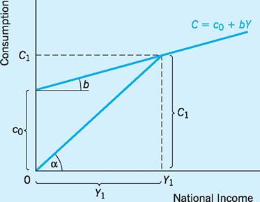
Fig. 16.1 The consumption function.
means that the proportion of income consumed (a.p.c.) falls. Indeed some early Keynesian economists were concerned that private sector investment would not grow as a proportion of income to fill the gap left by a declining average propensity to consume, in which case the economy would be subjected to ‘secular stagnation’.
For Keynes, the main influence on consumption in the short run was current disposable income, i.e. income minus direct taxes. When this fluctuated, so would consumption but, because the m.p.c. was less than 1, consumption would change by an amount less than the change in disposable income. If we look at the actual data for the UK and plot consumption against disposable income, both measured in real terms (using 2006 prices), we can see from Fig. 16.2 that over the period 1970-2009 there appears to be a close positive relationship between consumption and disposable income.2
In order to find numerical estimates for c0 and b for our consumption function, we can fit a regression line, or line of ‘best fit’,3 to the data in Table 16.1. Using linear regression we can derive the following equation:
C = -19,583 + 0.96Yd
where Yd is real disposable income (£m).
This consumption function (1970-2009) not only appears to fit the data well, as can be seen from Fig. 16.2, but also seems to support the Keynesian view that the m.p.c. is less than 1 (in our case 0.96). Somewhat surprisingly, the equation has a negative intercept of 19,583 (£m), implying that the a.p.c. rises as income rises. However, the intercept term is, statistically, not significantly different from zero and so we cannot be certain that the consumption function fails to go through the origin. If it did, this would mean that the a.p.c. does not rise as income rises.
As a first attempt, therefore, the above equation, which explains changes in consumption in terms of changes in current disposable income, seems to fit the facts and the Keynesian theory rather well. To take an example from Table 16.1, in 2006 real disposable income was £853,095m; fitting this into our equation gives predicted consumption of £799,388m. Actual consumption was £819,610m, an error of around 2%.
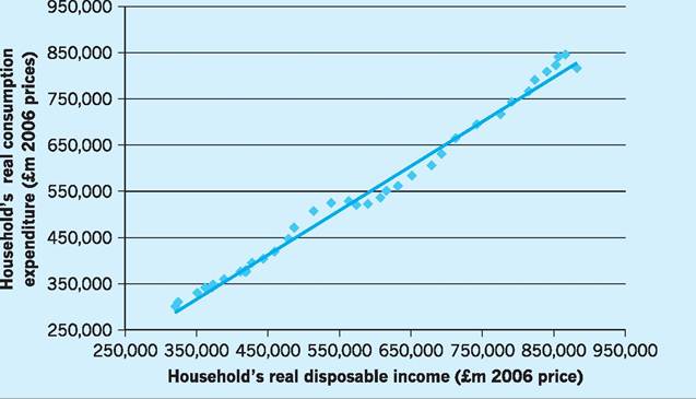
Fig. 16.2 The UK consumption-income relationship, 1970-2009.
Source: Based on Table 16.1.
Closer examination of the data, however, indicates that using changes in current disposable income to explain changes in consumption may be less than satisfactory. It may help to look more carefully at the ‘errors’, i.e. the deviations of the actual observations for consumption from the predicted values on the regression line. At first sight, these ‘errors’ in our earlier Fig. 16.2 do not look very large. Nevertheless, policy-makers relying on the simple consumption function equation to forecast any future consumption would, in some years, still make substantial errors. A more striking picture of the errors can be seen in Fig. 16.3. Here the differences between actual and forecast consumption, C = (-19,583 + 0.96Yd), are plotted.
Very large negative errors occurred from 1979 to 1982 and during much of the 1990s. In these periods actual consumption was very much less than forecast, given the levels of real disposable income. It appears that consumers were acting very cautiously because they were pessimistic about their future incomes. Such uncertainty was caused in part by oil-price shocks and rising unemployment. Similarly, in the early 1990s actual consumption was also lower than forecast by our equation, again in part because of uncertain future incomes as unemployment levels increased, but also because of falling asset prices (houses) and the desire of consumers to pay off accumulated debt.
The recent financial crisis in 2007/8, which also threatens jobs and house prices, has again caused a sharp fall in consumption as consumers react to uncertainty by saving and paying off debt.At the other extreme, large positive errors were made in the late 1980s and in the run up to the recent financial crisis in 2008. Here people actually consumed more than would be forecast by our equation, given the levels of real disposable income. This period was one of falling unemployment, inflated house prices and rising incomes, all of which made consumers more optimistic about the future.
It appears from the above that consumers are a good deal more sophisticated than the simple Keynesian consumption function would imply. Consumers take
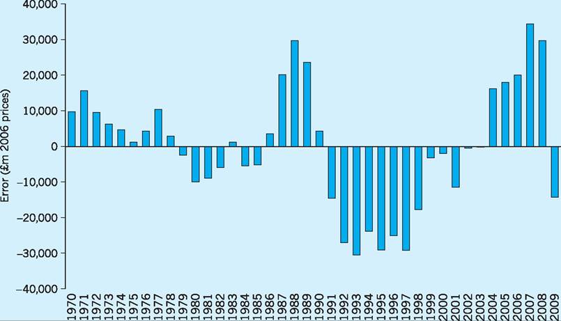
Fig. 16.3 Error analysis of simple consumption function (actual consumption minus forecast consumption).
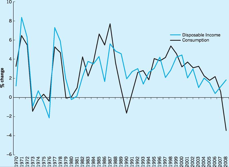
Fig. 16.4 UK annual percentage change in disposable income and consumption. Source: Based on Table 16.1.
into account not only their current income when deciding expenditure, but also their future expected income. Indeed one of the goals of the post-Keynesian theories of consumption considered in the next section is to attempt to include the influence of future income on consumer spending.
One other feature of consumer behaviour ought to be noted at this stage. In general, consumers attempt to keep a relatively smooth consumption pattern over the business cycle. In periods when disposable income is rising rapidly, consumption will rise but not in proportion. In other words, during the recovery period consumers behave cautiously, at least at first. Similarly, in periods when disposable income is falling, consumers will on the whole attempt to maintain their consumption as best they can despite their reduced circumstances. Put simply, in the short run, consumption usually fluctuates less than disposable income (i.e. the short-run m.p.c. is smaller than the long-run m.p.c.). Figure 16.4 illustrates this point for the UK, during the late 1970s.
Since the 1970s this pattern appears to have changed with consumption becoming more volatile than income. Financial deregulation and asset price inflation encouraged consumer borrowing in the mid- to late 1980s, which resulted in consumption increasing in those years by more than income. On the other hand, the severe recession of the early 1990s, coupled with the collapse of house prices and the hangover of indebtedness from the previous period, resulted in consumers cutting expenditure by more than income in an attempt to repay debt. It appears, therefore, that a Keynesian consumption function based only on current disposable income is insufficient to explain fully the short-run changes in consumer expenditure.
Post-Keynesian theories of the consumption function
The newer theories of the consumption function differed from that of Keynes in that they were more deeply rooted in the microeconomics of consumer behaviour. Two of the theories, Friedman’s Permanent Income Hypothesis (PIH) and Modigliani’s Life Cycle Hypothesis (LCH), start from the position that consumers plan their consumption expenditure not on the basis of income received during the current period, but rather on the basis of their long-run, or lifetime, income expectations.
In both these theories, therefore, the link between current consumption and current income is broken. A consumer determines his or her consumption for a given period on the basis of a longer-run view of the resources available, taking into account not just current income but future expected income and any change in the value of their assets. Of course, if consumers cannot borrow on the strength of future income, i.e. if they are liquidity constrained, then they will have to adjust current spending to current income, as in the Keynesian theory.
The Permanent Income Hypothesis (PIH)
In Friedman’s PIH an individual’s consumption is based on that individual’s permanent income (Yp). Technically Yp is defined as the return on the present value of an individual’s wealth, and hence it is what can be consumed whilst leaving the individual’s wealth intact. More generally Yp could be thought of as some form of long-run average income, or ‘normal income’, which can be counted on in the future. An individual’s actual or measured income (Y) in any time period will be made up of two parts - the ‘permanent’ part (Yp), and the ‘transitory’ part (Yt). Transitory income might be positive, if the individual is having an unexpectedly good year, or negative, if the individual is having a bad year. It follows that measured income is
Y = Yp + Yt
In the simplest form of the PIH, consumption is a constant proportion of permanent income, i.e.
C = kYp
where
k = F(i, w, x)
The proportion k is determined by factors such as the interest rate (i), the ratio of non-human to human wealth (w), and a catch-all variable (x) which includes age and tastes as a major component. If i rises, then individuals are assumed to feel more secure as to the future returns from their asset holdings, so that k increases. Equally, k will increase if the ratio of non-human to human wealth (w) rises in total wealth holding. This is also thought to increase individual security, since non-human wealth, such as money and shares, is assumed to be more reliable than human wealth, such as expected future labour income.
If the economy grows steadily, with no fluctuations, then Yp would be approximately equal to Y (measured National Income), and not only would a constant proportion of permanent income be consumed, but also a constant proportion of measured National Income. A study by Simon Kuznets (1946) in the US showed that if long-run data were used (10year averages of consumption and income) then the a.p.c. was roughly constant. Taking 10-year averages effectively eliminates short-run fluctuations in income, and so Kuznets’s results are consistent with the constant proportion k in the PIH.
This long-run consumption function derived from time-series data averaged over the business cycle, with its constant a.p.c., seemed, however, at odds with the short-run consumption function derived either from time-series data on an annual basis or from crosssectional data. The short-run consumption function was flatter than the long-run function (see Fig. 16.5), having therefore a lower m.p.c. and an a.p.c. that was not constant, falling when incomes rose (booms) and rising when incomes fell (slumps). The answer to this puzzle, according to Friedman, is that in booms more people will think that they are doing better than normal than will think they are doing worse than normal. For the economy as a whole, therefore, there will be positive transitory income (Yt), so that measured National Income (Y) will be above permanent income (Yp). The unexpectedly high measured income will, however, have little impact on consumer views of their permanent income unless it lasts for several years. Since consumer spending plans are based on permanent income, any boom that is not long-lived
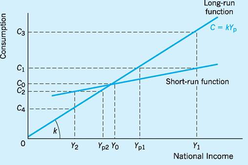
Fig. 16.5 Long- and short-run consumption functions.
will have little effect on consumer spending. The unexpected increases in income are therefore largely saved, with the result that in a boom the average propensity to consume falls. This is seen in Fig. 16.5.
As the economy expands along its long-run trend, consumption should be a fixed proportion, k, of income. In reality, however, the economy fluctuates around this long-run trend. Suppose we start in situation Y0, with measured and permanent income equal, consumption (kY0) equal to C0, and a.p.c. equal to k. The economy then experiences a boom with measured income rising to Y1. Permanent income will, however, be less affected by the sudden increase in income, and in our figure rises only to Yp1. Consumption, being based on permanent income, now rises to C1(kYp1). Only if measured income remained at Y1 for several years would permanent income be revised upwards to Y1, and consumption to C3(kY1). If this is not the case, then the proportion of income consumed will be only C1∕Y1, i.e. the a.p.c. will have fallen below the initial level k during the boom.
In a slump, income will fall, say from Y0 to Y2, and although permanent income may be revised downwards a little to Yp2, it will fall proportionately less than measured income. Consumption will therefore be C2(kYp2), falling much less than if Y2 had been regarded as permanent (when consumption would fall further to C4). The a.p.c. will then be C2∕Y2, which is above the initial level k.
It can be seen from this analysis that Friedman is able to explain why the short-run consumption function is flatter, with a variable a.p.c., whilst the long-run consumption function is steeper, with a constant a.p.c. Booms will, unless long-lived, cause a.p.c. to fall. There will be little upward revision of consumption plans, when higher income is largely regarded as transitory. Slumps will, unless long-lived, in a similar manner cause a.p.c. to rise.
The Life Cycle Hypothesis (LCH)
The LCH, developed by Modigliani and his associates, is similar in many ways to the PIH. Consumption is again seen as being a constant proportion k of Yp, with the same sort of variables affecting k as in Friedman’s theory. Modigliani stresses, however, the age of the consumer, with the consumer trying to even out consumption over a life-time in which income fluctuates widely. In youth and old age, when income is low, consumption is maintained by borrowing or drawing on past savings respectively, so that consumption is a high proportion of income; in middle life, when income is relatively high, a smaller proportion is onsumed, with savings being built up to finance consumption after retirement.
One of the empirical facts that needed to be explained by any theory was why, from cross-sectional data, it was seen that low-income groups had a higher a.p.c. than high-income groups. The LCH argued that low-income groups contain a high proportion of very young and very old households, both of which have a high propensity to consume. On the other hand, the high-income groups contain a high proportion of middle-aged households, with a low propensity to consume.
The variations in a.p.c. observed using time-series data, when National Income rises or falls, can also be explained by the LCH. Any windfall or transitory income received in a boom is spread over the individual’s remaining life-time. For example, an unexpected increase in income of, say, £1,000 for someone with 20 more years to live would mean that they would revise their Yp upwards by about £50 per annum, so that consumption in the year in which the windfall is received would increase by a relatively small amount (some proportion of £50). The a.p.c. would therefore fall with higher income because consumption (the numerator) will have risen by only a small amount, based on Yp, but measured income (the denominator) has risen by the full £1,000. An unexpected reduction in income in a recession would likewise be spread over an individual’s life-time, with borrowing and/or the running down of past savings leading to only a small cut in that individual’s current consumption, thereby causing a.p.c. to rise. The LCH has therefore been able, like the PIH, to reconcile the flatter short-run consumption function with the steeper long-run consumption function (with constant a.p.c.).
Both theories imply that the m.p.c., which is the slope of the consumption function, is lower in the short run than it is in the long run. In the PIH any unexpected increase in income is not consumed, but largely saved, whereas in the LCH it is spread over the consumer’s life-time. It follows that the multi- plier4 predicted by these theories will be small in the short run, because m.p.c. is low in the short run. Changes in government spending and taxation aimed at stabilizing the economy will therefore be relatively ineffective, especially if these changes are seen as being only temporary. A by-product of Friedman’s work on the consumption function appears, therefore, to be an attack on the effectiveness of Keynesian short-run demand-management policies.
The PIH and LCH appear to have broken the link between current consumption and current disposable income by arguing that consumption depends not only on current disposable income but also on all future disposable income. It could be argued, however, that there are two reasons why the influence of current income may be more important than these theories imply. First, it is unreasonable to believe that all consumers will be able to borrow and lend in different periods to even out their consumption pattern. An unemployed worker is unlikely to be able to borrow money to maintain his consumption, even though he is convinced he will be able to repay the loan out of future earnings. In this case, once past savings are exhausted, the constraint on consumption will be current disposable income. Second, estimates of future disposable income, on which permanent income is based, are highly uncertain. It is reasonable to expect, therefore, that the consumer uses his or her recent experience, and current income, as an important basis for estimating long-run or permanent income, and hence wealth. For both these reasons, therefore, one could still argue that current disposable income is still a major influence on current consumption, even under the PIH and LCH.
Rational expectations and consumption
The theories of consumption developed by Friedman, Modigliani and others all involve some concept of permanent or (long-term) ‘normal’ income on which households plan their consumption decisions. In order to arrive at this concept, households need to come to some view of their expected future income. The early post-Keynesian theories made convenient, if rather naive, assumptions about this process. Friedman, for example, used adaptive expectations, which means that consumers adapt or change their view of their expected income in the light of any ‘errors’ made in previous time periods. In effect it can then be shown that ‘permanent income’ (which is supposed to capture future expected income) is simply a weighted average of past incomes.
Despite the empirical convenience of this method of modelling expectations (data on past incomes being readily available), economists have become increasingly dissatisfied with this approach to modelling the formation of expectations. This approach is too mechanistic, is backward looking and, apart from income, ignores all other relevant information that might affect future earnings. As an alternative many economists have adopted the hypothesis of rational expectations. Rational expectation theory argues that households form expectations not only on the basis of past experience but also on their predictions about the future. It is assumed that households possess some sort of ‘model’ of the economy which they then use to process relevant information and derive an expectation of future income. Of course, most households do not possess any economic model of the economy. Nevertheless, forecasts from actual models are freely available in the media and households can use these, together with any specific knowledge they might have of their particular industry and region, to make a rational forecast of anticipated future income. Although economists have had problems in applying this concept of rational expectations to empirical work, much of the current theoretical study of consumption is based upon it.
One application of rational expectations to the permanent income model has been developed by Robert Hall. Hall (1978) argued that under certain conditions a household’s consumption should follow a ‘random walk,. If households have included all the available and relevant information in their forecast of future income then, assuming consumption smoothing, the only reason for a household to alter its consumption would be an unexpected change in income. Hence the best estimate of next year’s consumption (Ct+1) will be this year’s consumption (Ct), as this reflects all the available information on future incomes. That is to say, Ct+1 = Ct + et+1 where et+1 is a random amount that results from unexpected shocks. Hall found some evidence to support the view that next year’s consumption is closely related to this year’s consumption. However, he also found that other variables, including past income, influenced next year’s consumption. One reason for this finding is, of course, the linkage between past income and current borrowing potential for householders as a means of financing future consumption.
The substantial variations in the savings ratio over the last economic cycle have, to a large extent, been explained by the impact of monetary policy. Monetary policy, operating through the house price channel, in an environment of financial liberalization, has been held responsible for the boom-bust cycle. Work by Catao and Ramaswamy (1996), however, suggests that although the monetary stance and wealth effects on consumption accounted for over half the contraction in economic activity, the role of ‘true’ shocks also played a significant role. True shocks are defined as those that cannot easily be explained by obvious economic factors. These could be caused by pessimism about the future or anxiety about the particular course of political or social developments. One policy conclusion that comes from their work is that although monetary policy is influential, it is difficult for monetary policy to fine-tune the economy in the face of expectational shocks.
Windfall gains and consumption
In 1996 consumers received around £3.5bn in special payments, sometimes called windfall gains. In 1997 the figure was around £35bn. These windfall gains were mainly the result of the merger of building societies and their demutualization, which converted building society assets into tradeable shares. There were also windfall gains via enforced (by the regulator) payouts to customers from the regional electricity companies and the sums received from maturing TESSA accounts.
Economic theory tells us that an increase in a consumer’s wealth is unlikely to lead to a proportionate increase in consumption, with consumers maximizing utility by spreading the additional consumption over the rest of their life-time. The increase in current consumption is likely, therefore, to be relatively small. The Bank of England Inflation Report in February 1997 adopted this viewpoint, arguing that previous windfall payouts by the Abbey National and TSB had resulted in only modest increases in current consumption. The Bank of England estimated that only around 5-10% of the £35bn of windfall gains expected in 1997 would be spent in the first year (i.e. up to £3.5bn). This view was further supported by a survey carried out by the Harris Research Centre, which found that only 36% of individuals who expected to receive a building society windfall in 1997 intended to spend all or most of it.
Weale and Young (1998) found that the effect of the windfalls on consumption had turned out to be larger than the Bank of England had anticipated a year earlier. It was estimated that consumers’ expenditure in 1997 had risen by a further £8bn because of the windfall gains received in that year. One explanation might be that more consumers had suffered from liquidity constraints in 1997 than the Bank of England had anticipated. If an individual is liquidity constrained then arguably they cannot achieve their optimum consumption pattern taking into account expected future income because they cannot, for various reasons, borrow on the strength of that expected future income. Any liquidity-constrained consumer who receives a windfall gain is then likely to spend more of it in the current period than they would have done had no such liquidity constraint been present.
A study by Banerjee and Batini (2003) suggests that about one-seventh of UK consumers consume an amount equal to their current income. This result is obviously at odds with the PIH and the LCH but is consistent with evidence on credit restrictions in the UK. The authors also argue that it ties in with the evidence that consumption in the UK is more responsive to changes in human wealth (labour income) than the PIH would suggest.
I The savings ratio
Two motives for saving are usually identified, namely people save for precautionary reasons and for lifecycle reasons. The first motive involves households refraining from consuming all their income to build up a reserve for times when income is unexpectedly low. The second motive involves people needing to build up a reserve of savings during their working life to finance consumption during retirement.
Given these motives for saving there are several economic factors that are likely to influence the savings ratio (see Berry et al., 2009).
Permanent income
As we noticed previously, the permanent income/life cycle theory assumes households base their current consumption on some view of their permanent income over their whole life-time and that they would prefer a smooth consumption pattern. The forward-looking consumer will therefore save in periods when income is unexpectedly high (buying financial or housing assets) and will dis-save (selling assets or borrowing) when income is less than that expected in the future. The consumer boom and consequent fall in the savings ratio in the late 1980s and 1990s (see Fig. 16.6) was partly due to positive views about future income prospects (current income below permanent income).
Interest rates
The real rate of interest (nominal rate minus the expected inflation rate) is the main determinant of how much extra consumption can be obtained in the future by giving up consumption (saving) today. Higher real interest rates should therefore discourage consumption and borrowing and encourage saving, since still more extra consumption will result in the future by saving today. Higher real interest rates also redistribute income from borrowers to lenders. If lenders have a lower marginal propensity to consume than borrowers, then this will reduce consumption and raise the savings ratio. Expected changes in real interest rates should, by definition, have been taken into account by consumers but unexpected increases should raise the savings ratio. The unexpectedly low real interest rates (in some years negative) in the late 1970s and early 1980s are seen by many as having had a downward influence on the savings ratio at that time (see Fig. 16.6). The rise in real rates to its peak in 1990 is seen as having had the opposite effect.
Credit conditions
As argued earlier, some households are likely to be affected by liquidity constraints, i.e. they cannot borrow and spend as much as they would like to, based on their own perception of their future income. Any tightening of credit conditions, either quantitative (volume) or in price, is likely to increase the number of liquidity constrained households, reduce consumption and raise the savings ratio. The tightening of credit conditions and the reluctance of banks to lend whilst they rebuild their balance sheet positions after the recent financial crisis, is likely therefore to raise the savings ratio, as seems to have been the case since 2007 in Fig. 16.6.
Uncertainty
One motive for saving is to construct a buffer to support consumption when income unexpectedly falls. Any increase in economic uncertainty will, therefore, lead to a rise in precautionary saving. Any improvements in macroeconomic management which reduce economic fluctuations might then lead to less
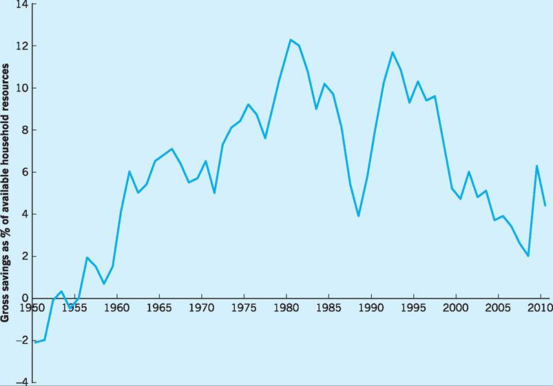
Fig. 16.6 UK households’ savings ratio (%). Source: ONS Economic Trends (various).
precautionary saving. The period of improved economic performance from the mid-1990s to 2007 might have helped reduce the savings ratio over that period.
Wealth
Non-human wealth, such as equities, house prices, etc., is part of a household’s life-time resources. Any increase in this wealth should therefore increase the amount of consumption out of any given level of income and thereby reduce the savings ratio. Most statistical studies, however, show that the m.p.c. related to changes in wealth is very low, about 0.04-0.06 (although estimates are subject to great uncertainty). The reasons why the low m.p.c. relates to changes in wealth are possibly to do with two main factors. First, the volatility of equity prices means that any increase in wealth linked to shares and other securities is not seen as permanent. Over half of household financial wealth is tied up in pension funds and life assurance and the effect of rising equity prices on these is not so obvious to consumers. However, house price inflation appears to be different; an increase (bad for people trading up but good for people trading down) seems to provide households with more collateral against which to borrow, and increased borrowing and spending will then lower the saving ratio. Second, because households can release equity from their house, if necessary, when income unexpectedly falls, rising equity prices reduce the need for precautionary savings. The fall in house prices 1990-93 coincided with a large (37%) rise in the savings ratio and may have been one contributory factor, and the same linkage seems to be a possible reason for the rise in the savings ratio post-2007.
Inflation
Inflation erodes the real value of the wealth that households hold; for example, bank and building society deposits, bonds, insurance policies and pension funds are all denominated in nominal terms and are eroded in real terms by inflation. In order to restore the real value of these assets, households have to save more. The savings ratio therefore tends to rise in times of high and unstable inflation, when nominal interest rates do not keep up with the increased inflation rate. Households therefore have to reduce consumption to increase their savings levels, and the savings ratio rises. The high savings ratios of the mid- to late-1970s and 1989-91 were associated with periods of high and unstable inflation.
Demographics
The life cycle theory of consumption suggests that the young on low income will be net borrowers (i.e. consume more than current income), people in their middle years will be net savers (to build up assets for retirement) and older retired people will run down their assets in order to consume. The demographic make-up of the population should therefore affect the overall household savings ratio. The UK post-war baby boom generation is now passing into retirement and this should therefore lower the savings ratio. On the other hand, the increase in life expectancy means a longer retirement period which may force workers in their middle years to save more, thus raising the ratio. These demographic factors only change slowly but do have a significant influence in the long term.
The savings of other sectors
Households are not the only savers in the economy. The corporate sector also saves when it retains profits. Governments save when they spend less than they receive in taxation, i.e. run a budget surplus. It is therefore the overall level of savings, national savings, that should be given close attention.
The theory of ‘Ricardian Equivalence’ sees private households and government savings as close substitutes for each other. If the government borrows (dissaves) to finance a tax cut, then households might expect higher future taxes and save the current tax cut. The household sector savings ratio therefore rises to compensate for the fall in the government savings ratio. Perversely, the government action which was intended to stimulate spending does no such thing! The theory assumes, of course, that households are forward-looking and are aware of, and concerned about, the implications of the government’s current budget surplus (savings) and its likely strategy as regards future tax liabilities! The theory is also undermined if a proportion of households are liquidity constrained, i.e. they are unable to borrow as much as they would wish in order to finance current consumption, based on their expected future earnings. If so, then any unexpected tax windfall will be used to raise consumption to the desired level rather than save the tax windfall.
The decline in the household savings ratio mid-1990s-2008
The UK savings ratio fell from 10.8% in 1993 to a low of 2% in 2008. Several reasons have been put forward for this decline. Benito et al. (2007) suggest that the fall in real interest rates during the period could account for about 4% points of the observed drop in the savings ratio. The fall in real interest rates was mainly explained by international factors, specifically the excess savings generated in emerging economies such as China and in the oil exporting countries.
The mid-1990s to the mid-2000s was also a period characterized by steady non-inflationary growth in the UK; the NICE (non-inflationary-continuous- expansion) decade, as Mervyn King, the Governor of the Bank of England, called it. The increased stability of the economy compared to previous decades may have encouraged households to save less for precautionary purposes.
From 2002/03 credit conditions in the UK became easier. The difference between the Bank Rate and mortgage lending rates declined, and the loan-to- income ratio on new mortgage lending rose (from 2.21 for first-time buyers in 1992 to 3.39 in 2007, according to the Council of Mortgage Lenders). Easier and cheaper credit encouraged consumers to bring forward consumption. Rising asset prices, especially house prices, may also have facilitated this process by providing householders with increased collateral against which to borrow. Interestingly, Berry et al. (2009) point out that although most of the benefit of asset price rises has gone to older households, it appears that younger households have reduced their saving most. Either asset prices do not play so much of a role in savings or perhaps there is an expectation of intergenerational transfers so that consumption occurs ahead of inherited income.
Two factors have influenced the savings ratio in the opposite direction. The increased numbers in their middle years over the period should have raised the savings ratio. In addition, companies with a defined benefit pension scheme made increased pension contributions on behalf of their employees, which are treated as household savings by the Office of National Statistics (ONS).
The international perspective
The fall in the household savings ratio over the period from the mid-1990s-2007 has been experienced across many countries (see Fig. 16.7). The influencing factors, namely low real interest rates, rising asset prices and improved economic stability, have been global. The variation in the magnitude of the impact, however, suggests that other factors were at play in different countries. For example, the increase in asset prices in the UK and US in the decade to 2007 did not occur in Germany, e.g. German house prices were 12% lower in real terms in 2007 compared to 1997.
The financial crisis and the savings ratio
The severe recession in 2008, the worst since the Second World War, caused house prices to fall, unemployment to rise and credit restrictions to be tightened, together with an increased uncertainty about the future stability of the economy. As we can see in Fig. 16.6, consumption fell and the savings ratio rose to 6.7% in 2009. The increase in the savings ratio and reduction in debt levels of households might be desirable at an individual level, but might make economic recovery more difficult, i.e. the so-called ‘paradox of thrift’.
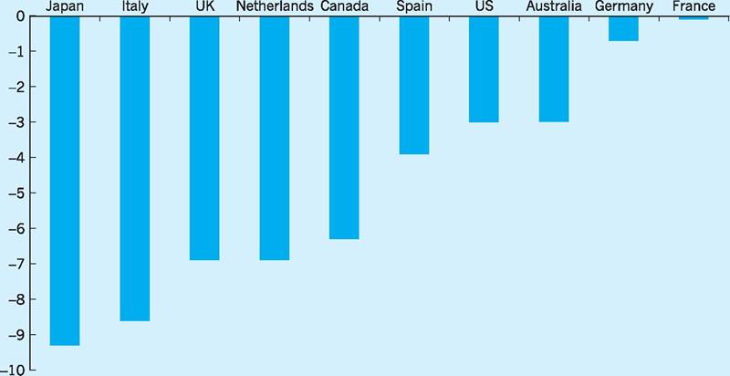
Fig. 16.7 Percentage points change in household savings ratio between average for 1992-97 and average for 2003-08.
Source: ONS Economic Trends (various).
Table 16.2 National and sectoral savings and investment.
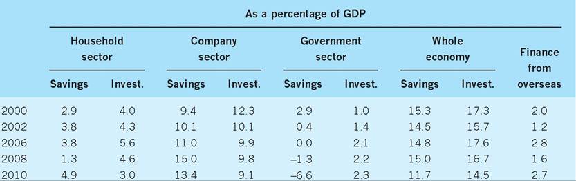
Source: National Institute Economic Review (2010), July, No. 213, Table A9, p. 165.
National saving
National saving is the sum of saving by the public and private sectors. Table 16.2 illustrates the savings of the various sectors as a percentage of GDP. Overall, if the amount that is invested by a country exceeds the amount that is saved then the excess is represented by the financial account deficit on the balance of payments. In 2008 Britain’s national savings rate of 15.8% was lower than that of any other OECD country except Iceland (6.1%), Greece (7.1%), Portugal (10.2%) and the US (12.1%). It may be relevant to ask the question: is Britain’s savings rate too low? Britain does not have the same requirement to save as, say, Germany (25.8%) or Italy (18.0%) with their rapidly ageing populations. However, as pointed out in the National Institute Economic Review, over the last 20 years the low national savings ratio in the UK has constrained investment and hence wealth formation. Wealth has fallen as a percentage of income and the effects are visible in terms of low levels of public infrastructure and high house prices, both in part the consequence of not generating enough savings to be invested in these forms of capital.
Indeed, a recent study by Weale (2009) calculates the level of savings required by each cohort to fund its consumption without reliance on transfers from other generations, what he calls ‘savings adequacy’. Given realistic estimates of real interest rates and economic growth, he concludes that current consumption patterns are unaffordable, both for the current adult population (can ‘afford’ only 88.8% of their current consumption) or more importantly for people starting their adult life (can ‘afford’ 89.3%). Weale sees the only solutions as increasing labour income, either by increased employment rates or longer working lives, or by relying on transfers from younger generation to those not working.
Savings attracted from abroad have helped UK investment to exceed UK savings. However, this implies future payments of net property income abroad, with a negative impact on the UK balance of payments. It follows that the current excess of world savings is not a reason for the UK to avoid facing up to its savings gap!
I Conclusion
The importance of having a clear idea of what factors determine consumption cannot be overestimated. Consumption expenditure is the largest element in total expenditure and so any fluctuations in consumption will have important implications for the overall level of demand in the economy. The failure to appreciate the strength of consumer demand in 1987 and 1988 was an important contributory factor to the subsequent deterioration in the inflation and balance of payments position that has posed such problems for the UK economy. Similarly the fall in consumer spending in the recession of the early 1990s was much sharper than in either of the previous two recessions of 1974-77 and 1979-82. Again this change in consumption expenditure was largely unforeseen by forecasters.
Post-Keynesian theories stress that, when deciding on consumption, consumers have a longer-term planning horizon than merely considering current income, the implication of post-Keynesian theories being that consumption is more stable than Keynesians thought. Evidence suggests, however, that in the face of uncertainty and liquidity constraints, current income may still be a key factor influencing consumption.
Changes in savings rates have both a short-run impact on aggregate demand and a long-run impact on future wealth and consumption.
Key points
■ In the Keynesian view, current disposable income is the main determinant of consumer spending.
■ The suggestion here is that the average propensity to consume (a.p.c.) will fall as disposable income increases.
■ Further, the marginal propensity to consume (m.p.c.) will be less than 1.
■ Using a line of ‘best fit’ to UK data over the period 1970-2009, the consumption function has been estimated as C = -191,583 + 0.96Yd, where Yd is real disposable income (£m).
■ This suggests an m.p.c. of 0.96 and a negative intercept term, suggesting a.p.c. will rise, but only slightly, as disposable income increases.
■ Evidence began to accumulate that the short-run consumption function was flatter than the long-run consumption function. In other words, short-run m.p.c. is less than long-run m.p.c.
■ Attempts to explain this discrepancy have resulted in independent variables other than current disposable income being proposed. The Permanent Income Hypothesis (Friedman) and Life Cycle Income Hypothesis (Modigliani) have been suggested.
■ Even models based on past experience and future expectations have been used (rational expectations).
■ The policy consequences of errors in forecasting consumption (and therefore savings) are serious: underestimates of consumption cause economic policy to be over-expansionary (inflationary); overestimates of consumption cause economic policy to be over-cautious (deflationary).
■ Savings rates have both short-run and long-run effects on the economy.
Now try the self-check questions for this chapter on the Companion Website. You will also find useful links to relevant websites.
Notes
1 This is a ‘generalized’ version of the Keynesian consumption function as it uses total income rather than disposable income as the independent variable.
2 However, this is not always the case, as can be seen on the rare occasions when m.p.c. is negative. A negative m.p.c. means that when disposable income falls, consumption actually rises. In 1975, 1976, 1980, 1981, 1991 and 2009, the m.p.c. was indeed negative (Table 16.1).
3 ‘Best’ in the sense that it minimizes the sum of squared deviations from the line.
4 The simple National Income multiplier is defined as 1/1 - m.p.c. for a closed economy with no government sector, and indicates the extent to which National Income changes following a given change in injections or withdrawals. If m.p.c. is low, the multiplier is low.
References and further reading
Banerjee, R. and Batini, N. (2003) UK consumers’ habits, External MPC Unit Discussion Paper, No. 13, London, Bank of England.
Benassy-Quere, A. and Coeure, B. (2010) Economic Policy, Oxford, Oxford University Press.
Benito, A., Waldron, M., Young, G. and Zampolli, F. (2007) The role of household debt and balance sheets in the monetary transmission mechanism, Bank of England Quarterly Bulletin, 47(1): 70-8.
Berry, S., Williams, R. and Waldron, M. (2009) Household savings, Bank of England Quarterly Bulletin, 49(3).
Catao, L. and Ramaswamy, R. (1996) Recession and recovery in the United Kingdom in the 1990s: identifying the shocks, National Institute Economic Review, 157(July): 97-106.
Chrystal, A. K. (1992) The fall and rise of saving, National Westminster Bank Quarterly Review, February, 24-40.
Giavazzi, F. and Blanchard, O. (2010) Macroeconomics: A European Perspective, Harlow, Financial Times/Prentice Hall. Goldsmith, E. (2009) Consumer Economics: Issues and Behaviours (2nd edn), Oxford, Oxford University Press.
Hall, R. (1978) Stochastic implications of the life cycle permanent income hypothesis, Journal of Political Economy, 86(December): 971-87. Kennally, G. (1985) Committed and discretionary saving of households, National Institute Economic Review, 112(May): 35-40.
Keynes, J. M. (1936) The General Theory of Employment, Interest and Money, Basingstoke, Macmillan.
Kuznets, S. (1946) The National Product Since 1869, Cambridge, MA, The National Bureau of Economic Research.
Leighton Thomas, R. (1984) The consumption function, in D. Demery, et al. (eds),
Macroeconomics, Surveys in Economics, Harlow, Longman.
National Institute Economic Review (2010) 213, July.
OECD (2010) Economic Outlook, No. 87, July, Paris, Organisation for Economic Cooperation and Development.
Weale, M. (2009) Saving and the National Economy, Discussion Paper 340, September, London, National Institute of Economic and Social Research.
Weale, M. and Young, G. (1998) Debt Management, National Institute Economic Review, April.