DENSITY ESTIMATION

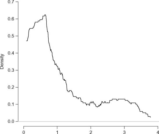
The analysis of a probability density function is a powerful tool to describe several prop­erties of a variable of interest. For instance, Figure 6.2 shows the estimated density func­tion of GDP per capita in 121 countries across the world in 1988.7 We can see that the density function is bimodal.

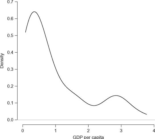
Figure 6.2 Kernel density estimation of GDP per capita in 121 countries normalized by the global mean.

⁷ The data are unweighted (each country as equal weight) and are taken from the Penn World Table of Summers and Heston (1991). The horizontal axis is the per capita GDP for each country normalized by the (unweighted) mean over all countries.

available from the full distribution of a variable than the restricted information provided by standard descriptive statistics, as the mean, variance, skewness, or kurtosis, which sum­marize each limited properties of the distribution on single values.

In the multivariate case, the conditional density function can provide useful insights on the relationship between several variables.

In practice, the functional form of the density function is often unknown and has to be estimated. For a long time, the main estimation method was mainly parametric. How­ever, a parametric density estimation requires the choice of a functional form a priori, and most of them do not fit multimodal distribution. In the last two decades, nonparametric and semiparametric estimation methods have been extensively developed. They are often used in empirical studies now and allow us to relax the specific assumptions underlying parametric estimation method, but they require in general more data on hand.

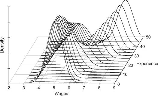
Figure 6.3 Conditional density estimates of wages on experience.

In this section, we will present parametric, nonparametric, and semiparametric den­sity estimation methods. Standard parametric methods are presented in Section 6.3.1, kernel density methods in Section 6.3.2, and finite mixture models in Section 6.3.3.

6.3.1 Parametric Estimation

We say that a random variable Y has a probability density function/, if the probability that

Y falls between a and b is defined as:

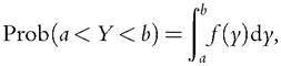
where a and b are real values and a < b.

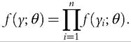
A parametric estimation requires one to specify a priori a functional form of the density function, that is, to know the density function up to some parameters. The density func­tion can then be written f(y; θ), where θ is a vector of k unknown parameters and y a vector of n observations. The problem remains of estimating θ; this is usually done by maximizing the likelihood to observe the actual values in a sample. If the data are inde­pendent and identically distributed (IID), the joint density function of n observations y₁, y₂, ■ ■ ■, y_n is equal to the product of the individual densities:

The estimation of the density function therefore requires the maximization of this func­tion with respect to θ. Because the logarithmic function is positive and monotone, it is equivalent to maximize

from which the solution is often much simpler. This estimation method is known as the maximum likelihood method.

6.3.1.1 Pareto

Pareto (1895) initiated the modeling of income distribution with a probability density function^[187] that is still in common use for modeling the upper tail of income and wealth distributions. Beyond a minimal income, he observed a linear relationship between the logarithm of the proportion of individuals with incomes above a given level and the

logarithm of this given level of income. This observation has been made in many situ­ations and suggests a distribution that decays like a power function; such behavior char­acterizes a heavy-tailed distribution.¹⁰ The Pareto CDF is given by

with density

where A :=y“.

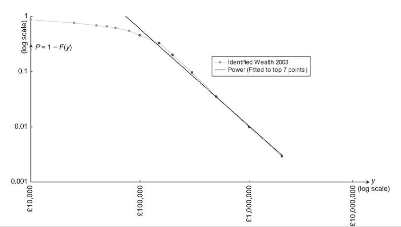
Figure 6.4 Pareto distribution. UK Identified wealth 2003. Source: Inland Revenue Statistics 2006, Table 13.1.

^[1] A “heavy-tailed” distribution F is one for which lim₇!∞e^λy[1 — F(y)] = ∞, for all λ > 0: it has a tail that is heavier than the exponential.

6.3.1.2 Lognormal

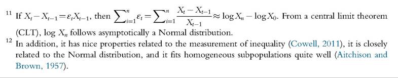
Gibrat (1931) highlighted the central place of the lognormal distribution in many eco­nomic situations. His law of proportionate effect says that if the variation of a variable between two successive periods of time is a random proportion of the variable at the first period, then the variable follows a lognormal distribution.¹¹ He successfully fitted log­normal distributions with many different data sets, as for instance income, food expen­ditures, wages, bequests, rents, real estate, firm profits, firm size, family size, and city size. The lognormal distribution has then been very popular in empirical work¹² and is often appropriate for studies of wages—see Figure 6.5. However, the fit of the upper tail of more broadly based income distributions appears to be quite poor. The tail of the log­normal distribution decays faster than the Pareto distribution, at the rate of an exponential function rather than of a power function. It has led to the use of other distributions with two to five parameters to get a better fit of the data over the entire distribution.

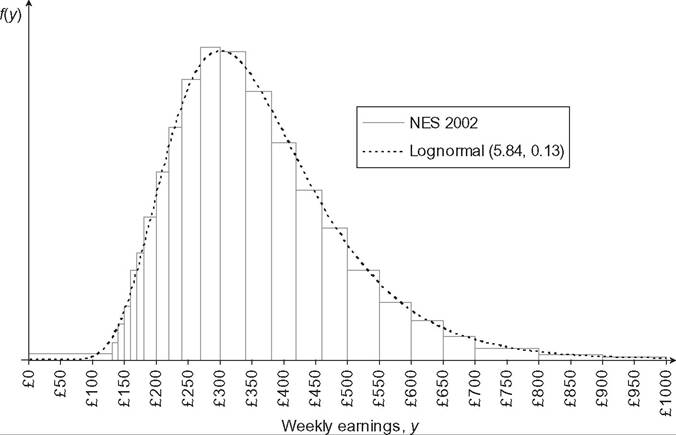
Figure 6.5 Lognormal distribution.

6.3.1.3 GeneralizedBeta

The gamma and Weibull distributions have shown good fit in empirical studies.^[188] The lognormal, gamma, and Weibull density functions are two-parameter distributions; they share the property that Lorenz curves do not intersect, contrary to what is observed in several datasets. To allow intersecting Lorenz curves, three-parameter distributions should be used, as the generalized gamma (GG), Singh-Maddala (SM), and Dagum dis­tributions.^[189] [190] ¹⁵ As shown by McDonald and Xu (1995), all the previously mentioned dis­tributions are special or limiting cases of the five-parameter generalized beta distribution, defined by the following density function:

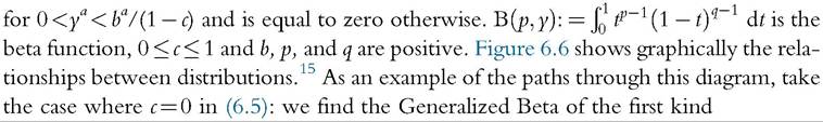
Figure 6.6 Parametric distributions tree. Source: Bandourian et al., 2003.

I distribution (6.3). Formore details on continuous univariate distributions, see Johnson et al. (1994) and Kleiber and Kotz (2003).

Income distributions have been extensively estimated with parametric density func­tions in the literature; see, for instance, Singh and Maddala (1976), Dagum (1977, 1980, 1983), McDonald (1984), Butler and McDonald (1989), Majumder and Chakravarty (1990), McDonald and Xu (1995), Bantilan et al. (1995), Victoria-Feser (1995, 2000), Brachmann et al. (1996), Bordley et al. (1997), Tachibanaki et al. (1997), and Bandourian et al. (2003). In most of these empirical studies, the generalized beta of the second kind, the Singh-Maddala and the Dagum distributions perform better than other two/three- parameter distributions.

6.3.1.4 GoodnessofFit

Goodness-of-fit test statistics are used to test whether a given sample of data is drawn from an estimated probability distribution. They are used to know if an estimated density func­tion is appropriate and fits the data well. Several statistics have been proposed in the lit- val, E_i is the expected percentage in the ith histogram interval, and m is the number of histogram intervals. This measure summarizes discrepancies between frequencies given by a histogram obtained from the data and those expected from the estimated density function. A statistic not significantly different from zero suggests that the estimated den­sity function fits well the unknown density function that generated the data. In finite sam­ples, this statistic is known to have poor finite sample power properties, that is, to underreject when the estimated density function is not appropriate; see Stephens (1986). Then the Pearson chi-square test isusually not recommended as a goodness- where ι(∙) is the indicator function defined in (6.1). When the observations are indepen­dently and identically distributed, it is a consistent estimator of the CDF. EDF-based sta­tistics measure the discrepancy between the EDF and the estimated CDF. They are not sensitive to the choice of the histogram’s bins as in the Pearson chi-squared statistic. For instance, the Kolmogorov-Smirnov statistic is equal to

where w(y) is a weighting function. The Cramer-von Mises statistic corresponds to the special case w(y) = 1, while the Anderson-Darling statistic puts more weight in the tails, withIn finite samples, the Anderson-Darling test sta­

tistic outperforms the Cramee r-von Mises statistic, which in turn outperforms the Kolmogorov-Smirnov test statistic, see Stephens (1986).

In distributional analysis, goodness-of-fit test statistics and inequality measures do not usually share the same intellectual foundation. The former are based on purely statistical criteria, whereas the latter are typically based on an axiomatic that may be associated with social welfare analysis or other formal representations of inequality in the abstract. Cowell et al. (2014) developed a family of goodness-of-fit tests founded on standard tools from the economic analysis of income distributions, defined as:

^[1] See Cowell et al. (2013) for an extension to the choice of any other “reference” distribution, giving for instance inequality measures telling us how far an empirical distribution is from the most unequal distribution.

estimated parametric distribution.¹⁷ It has excellent size and power properties as com­pared with other, commonly used, goodness-of-fit tests. It has the further advantage that the profile of the Gξ statistic as a function of ξ can provide valuable information about the nature of the departure from the target family of distributions, when that family is wrongly specified.

6.3.2 Kernel Method

6.3.2.1 From Histogram to Kernel Estimator

Histograms are the most widely used nonparametric density estimators. However, they have several drawbacks that kernel density method allows us to handle.

Figure 6.7 illustrates several problems arising with histograms, using GDP per capita in 121 countries in 1988 (solid line). The left plot is given with five bins of the same length between 0 and 5. The middle plot is similar but the position of the bins has changed; they are between —0.5 and 4.5. The two pictures are very different, even if they estimate the same distribution. The left panel shows a unimodal distribution, whereas the middle panel shows a bimodal distribution. Histograms are then sensitive to the point at which we start drawing bins. The right panel is given with 10 bins of the same length between 0 and 5. Once again, it gives a different picture of the same distribution. Histo­grams are thus sensitive to the number of bins used, which is also relatively arbitrary. Moreover, and most obviously, the pictures given by histograms provide discontinuities at the edge of each bin, which may not be an appropriate property of the true underlying distribution.

To avoid having to make an arbitrary choice on the position and the number of bins, we can use intervals that may overlap, rather than being separate from each other. The principle here is to estimate a density function at one point by counting the number of observations that are close to this evaluation point. For a sample of n observations, y₁,..., y_n, the naive density estimator is given by:

where h is the width of the intervals and ι(∙) is the indicator function (6.1). In this equa­tion, the estimate of the density at point y is given by the proportion of observations that

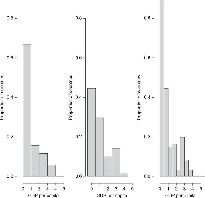
Figure 6.7 Histogram's sensitivity to the position and the number of bins.

are within a distance of h/2 or less from point y. The global density is obtained by sliding this window of width h along all the evaluation points.

Figure 6.8 presents the naive estimation of the density of GDP per capita across dif­ferent countries in 1988. Compared to histograms, the naive estimator reveals much more detail about the curvature of the density function. However, discontinuities are still present.

The kernel estimator is a generalization of the naive estimator, which allows us to overcome the problem of differentiability at all points. The discontinuity problem comes from the indicator function ι(∙), which allocates a weight of one to all the observations that belong to the interval centered on y and zero weight to the other observations. The principle of kernel estimation is simple: Rather than giving all observations in the interval the same weight, the allocated weight is greater the closer the observation is to y. The

GDP per capita

Figure 6.8 Naive estimator of GDP per capita.

transition from 1 to 0 in the weights is then carried out gradually, rather than abruptly. The kernel estimator is obtained by replacing the indicator function by a kernel function K(∙):

Forf (y) to conserve the properties of a density function, the integral of the kernel func­tion over the entire space has to be equal to one. Any probability distribution can then be used as kernel function. The Gaussian and the Epanechnikov distributions are two ker­nels commonly used in practice.¹⁸ Kernel density estimation is known to be sensitive to the choice of the bandwidth h, whereas it is not really affected by the choice of the kernel function.

6.3.2.2 Bandwidth Selection

The question of which value of h is the most appropriate is particularly a thorny one, even if automatic bandwidth selection procedures are often used in practice. Silverman’s rule of thumb is mostly used, which is defined as follows:¹

where σ is the standard deviation of the data, and q₃ and ^₁ are, respectively, the third and first quartiles calculated from the data. This rule boils down to using the minimum of two estimated measures of dispersion: the variance, which is sensitive to outliers, and the interquartile range. It is derived from the minimization of an approximation of the mean integrated squared error (MISE), a measure of discrepancy between the estimated and the true densities, where the Gaussian distribution is used as a reference distribution. This rule works well in numerous cases. Nonetheless, it tends to oversmooth the distribution when the true density is far from the Gaussian distribution, for example if it is multimodal and highly skewed. Figure 6.2 is a kernel density estimation of GDP per capita with Silver­man’s rule-of-thumb bandwidth selection. It appears as a smoothed version of the naive estimator in Figure 6.8. Several other data-driven methods for selecting the bandwidth have been developed such as cross-validation (CV) (Bowman, 1984; Rudemo, 1982; Stone, 1974) and plug-in methods (Ruppert et al., 1995; Sheather and Jones, 1991), among others.

Rather than using a Gaussian reference distribution in the approximation of the MISE, the plug-in approach consists of using a prior nonparametric estimate, and then choosing the h that minimizes this function. This choice of bandwidth does not then produce an empirical rule as simple as that proposed by Silverman, as it requires numerical calculation. For more details, see Sheather and Jones (1991).

Rather than minimizing the MISE, the underlying idea of CV by least squares is to minimize the integrated squared error (ISE). In other words, we use the same cri­terion, but not expressed in terms of expectations. The advantage of the ISE criterion is that it provides an optimal formula for h for a given sample. The counterpart is that two samples drawn from the same density will lead to two different optimal band­width choices. The ISE solution consists in finding the value of h that minimizes: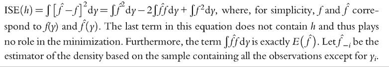

19

See Equation (3.31) in Silverman (1986, p. 48).

6.3.2.3 Adaptive Kernel Estimator

In the kernel density estimation presented earlier, the bandwidth remains constant at all points where the distribution is estimated. This constraint can be particularly onerous when the concentration of data is markedly heterogeneous in the sample. There would be advantages to using narrower bandwidths in dense parts of the distribution (the mid­dle) and wider ones in the more sparse parts (the tails). The adaptive kernel estimator is defined as follows:

Figure 6.9 presents the adaptive kernel density estimation of GDP per capita across different countries in 1988. Compared to the simple kernel density estimation, with fixed bandwidth (dashed line), the first mode is higher, and the second mode lower.

Several empirical studies on income distribution have used kernel density estima­tion, among others, see Marron and Schmitz (1992), Jenkins (1995), Cowell et al. (1996), Daly et al. (1997), Quah (1997), Burkhauser et al. (1999), Bourguignon and Morrisson (2002), Pittau and Zelli (2004), Jenkins and Van Kerm (2005), and Sala-i- Martin (2006).

²⁰ In practice, an initial fixed-bandwidth kernel estimator can be employed as f(yi), with θ = 1/2 and λ obtained with Silverman’s rule of thumb.

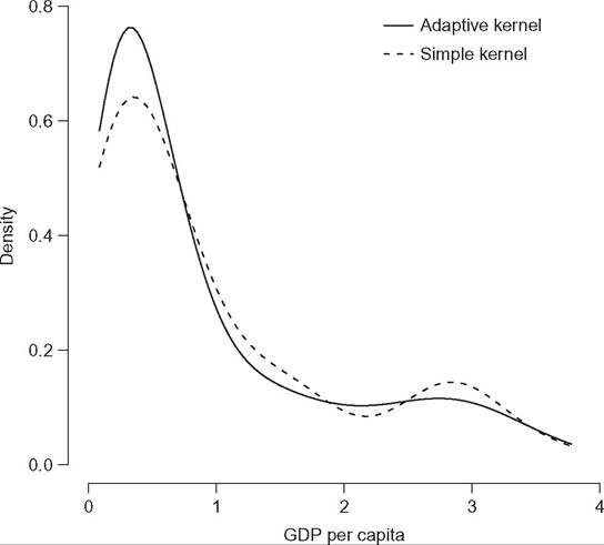
Figure 6.9 Adaptive kernel estimation of GDP per capita.

6.3.2.4 Multivariate and Conditional Density

The extension to the multivariate case is straightforward. Thejoint density of two vari­ables y and x, for which we have n observations, can be estimated with a bivariate kernel function

which is equivalent to the product of two univariate kernels in the Gaussian case. The extension to the d-dimensional case is immediate, via the use of multivariate kernels in d-dimensions. Scott (1992) extends Silverman’s rule of thumb as follows:

, where σ₁ and σ₂ are the sample standard deviations of, respectively, y and x. In practice, kernel density estimation is rarely used with more than two dimen­sions. With three or more dimensions, not only may the graphical representation be problematic, but the precision ofthe estimation may be also. Silverman (1986) showed that the number of observations required to guarantee a certain degree of reliability rises explosively with the number of dimensions. This problem is known as the curse of dimensionality.

A conditional density function is equal to the ratio of a joint distribution and a mar­ginal distribution,f(y∣x) = f(x,y~)∕f(x). A kernel conditional density estimation is then given by

When several conditional variables are considered, the bandwidth selection obtained by CV can mitigate the curse of dimensionality problem if some of them are irrelevant (Fan and Yim, 2004; Hall et al., 2004). Several recent studies have focused on conditional anal­ysis in a nonparametric framework. To evaluate policy effects, the impact of a counter- factual change in the distribution of some covariates on the unconditional distribution of some variable of interest has been investigated in DiNardo et al. (1996), Donald et al. (2000), Chernozhukov et al. (2009), Rothe (2010), and Donald et al. (2012). For more details on kernel density estimation, see Silverman (1986), Paul (1999), Li and Racine (2006), and Ahamada and Flachaire (2010).

6.3.3 Finite Mixture Models

6.3.3.1 A Group Decomposition Approach

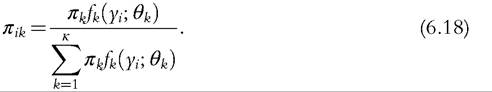
A population can be decomposed into several distinct groups in many different ways. The density function of the population is then equal to the sum of the densities associated with each of the different groups. Let us consider κ groups, with the density function of each grates to one over the support. A density estimation by mixture models is obtained by replacing the unknown parameters by estimated parameters. In finite mixture models, the group to which each individual belongs is not observed.²¹ They thus allow us to cap­ture the effect of unobserved heterogeneity. They can also be used for classification pur­pose. Bayes’ theorem allows us to deduce the a posteriori probability that an observation i belongs to the group k:

²¹ When the groups are known and also the densities associated to each groups, the mixture model is entirely parametric and can be estimated by maximum likelihood (see Section 6.3.1).

Replacing the unknown parameters by consistent estimates, these individual probabilities can be used to classify the observations into the different groups.

The estimation of a density by a mixture model allows us to bring out the link between parametric and nonparametric estimation. If we consider one single group (κ = 1), then the mixture models amount to just one parametric function. Adding addi­tional groups allows us to estimate more complicated densities, which cannot be modeled with one sole group; adding more groups allows us to reflect the heterogeneity of the population. Mixture models thus permit much greater modeling flexibility. In the extreme case, where we have as many groups as we do observations (κ = n), the mixture is equivalent to the estimation of a density by kernel methods (see Section 6.3.2).²² For values of κ between 1 and the size of the sample n, the mixture model can thus be seen as a semiparametric compromise between parametric estimation and nonparametric kernel estimation. The parametric aspect is reflected in the fact that the density is expressed as a sum of parametric density functions; the nonparametric aspect is captured by the pres­ence of a number of different groups.

The theory of mixture models tells us that, under regularity conditions, any proba­bility density can be consistently estimated as a mixture of Normal distributions.²³ Figure 6.10 depicts a number of different mixtures of two Normal distributions, of density and the two individual components are represented in the same figure.²⁴ From global densities (solid lines), we can see that a wide variety of densities can be represented by a mixture of only two Normal distributions, as top flat (panel a), bimodal (panel b), skewed (panel c), and thick upper-tailed (panel d) distributions. Many further examples can be provided to illustrate the very wide variety of distributions that can be character­ized by a mixture of κ Normal distributions: see, among others, Marron and Wand (1992). All these examples reveal the great flexibility of finite mixture models in estimat­ing densities.

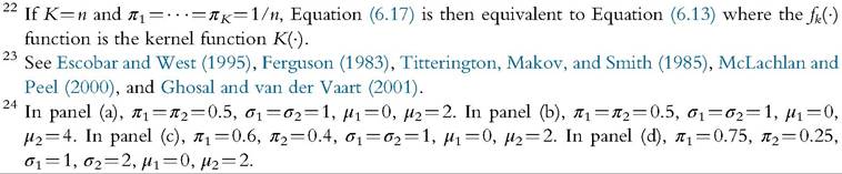
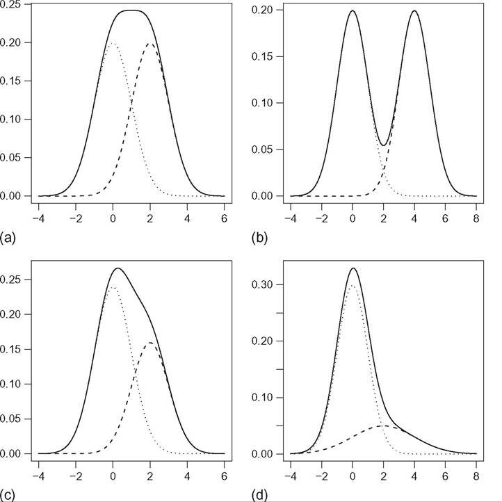
Figure 6.10 Mixtures of two Normal distributions.

6.3.3.2 Number of Components and Number of Groups

For a given number of κ, we can estimate the unknown parameters by maximum likelihood.^[191] The number κ, known as the number of components, can be selected by minimizing a criterion, as the Bayesian Information Criterion (BIC),

where ‘ is the estimated log-likelihood, #param is the number of parameters to estimate, and n is the number of observations. If the main concern is the best fit of the overall den­sity, this selection criterion is appropriate. However, if the main concern is the detection of distinct groups, the choice of κ is less simple. Indeed, there is no automatic correspon­dence between the choice of κ and the number of underlying groups in the population. Forinstance, panel (d) in Figure 6.10 shows that the second component is required to fit a thick upper tail, but it does not clearly identify a distinct group from the first component. Indeed, the two distributions of the groups intersect a lot. Here, the number of compo­nent κ is not necessarily equivalent to the number of groups. It illustrates that the defi­nition of what constitutes a distinct group and its detection can be a difficult task in finite mixture models.^[192]

Figure 6.11 shows kernel density estimation (on the left) and estimation by a mix­ture of lognormal distributions (on the right) of the income distribution in the

Figure 6.11 Income distribution in the United Kingdom in 1973 (incomes normalized by contemporary mean).

United Kingdom in 1973. A lognormal distribution is heavy tailed, in the sense that it has an upper tail that is heavier than an exponential. Then, it is more appropriate to use finite mixtures of lognormals rather than finite mixture of normals to fit income distributions, which are typically heavy tailed. The estimation of the density by a mixture of lognormal distributions is obtained from an estimation of the density of log-incomes by a mixture of Normal distributions.²⁷ The value of the bandwidth given by Silverman’s empirical rule (h = 0.08559) allows us to reproduce the kernel density estimation results in Marron and Schmitz (1992). Kernel estimation with a smaller value of h(0.01) are overlaid in the same figure. The comparison of the two estimators reveals that the results differ significantly: with h = 0.08559, the first mode is smaller than the second, whereas with h = 0.01 the reverse holds. This confirms that the kernel estimation with Silverman’s rule of thumb does indeed tend to oversmooth the function when the underlying distribution is multimodal and highly skewed distribution (see Section 6.3.2). In our example, the Silverman selection choice tends to flatten out considerably the first mode relative to the second. The right panel shows the density estimation with a mixture of lognormal distributions, obtained by minimizing the BIC. The overall distribution appears to be a smoothed representation of the kernel density estimation with h = 0.01. In addition, the mixture estimation identifies three separate components. The first and the third com­ponents do not overlap a lot; they can be associated to two distinct modes. The second component overlaps to a considerable extent with the third and to a lesser extent with the first. The presence of this second component allows a better fit of the right-hand side tail of the distribution, but cannot be clearly associated to a distinct group.

A very few empirical studies have used finite mixture models to estimate income dis­tributions. Flachaire and Nuiiez (2007) studied the distribution of household income in the United Kingdom with a mixture of lognormal distributions. Pittau and Zelli (2006) and Pittau et al. (2010) studied the evolution of per capita income distributions across EU regions and countries. Chotikapanich and Griffiths (2008) estimated the Canadian income distribution using a mixture of Gamma distributions. Lubrano and Ndoye (2011) modeled the income distribution using a Bayesian approach and a mixture of log­normal densities.²⁸

6.3.3.3 Group Profiles Explanation

In addition to the estimate of a density function of any form, finite mixture estimation can be used to explain the profiles of the different groups underlying the overall population. This can be done by introducing covariates in the probabilities π_k:

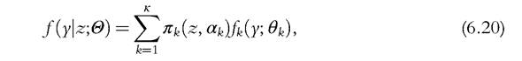
where z = {z₁,..., z_l} is a vector of l observed variables and

vector of l unknown parameters. This model defines a conditional density function, which takes into account directly the fact that the probability of group membership may be a function of individual characteristics (a white-collar worker has a greater prob­ability of belonging to the group of the richest households than does a blue-collar worker). As well as the nonparametric estimation of the density and the decomposition into different groups, covariates also explain the variability between groups. The rela­tionship between the probabilitiesand the covariates z can be specified with an ordered logit/probit or multinomial regression model, and the unconditional density can be obtained as follows:

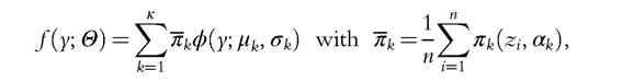
where z_i represents the vector of characteristics of the ith observation, and n is the number of observations. In other words,is the probability that the individual i with

characteristics z_i belong to the group k. For more details, see Ahamada and Flachaire (2010).

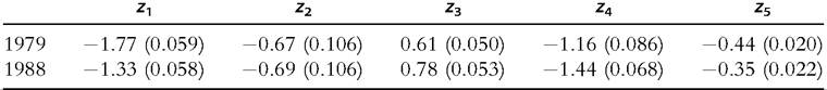
Figure 6.12 reproduces the results of the estimation of the distribution of household income in the United Kingdom in 1979 and 1988, obtained in Flachaire and Nuhez (2007), by a mixture of lognormal distributions.²⁹ The decomposition into groups of the mixture estimator does emphasize clear changes over time that would be difficult to see from the comparisons of the overall distributions. The analysis by groups shows that, in 1988, a small separate group had formed to the extreme left of the distribution, whereas that situated to the far right of the distribution had grown in size. Table 6.3 reproduces the estimated coefficients (with standard errors in parentheses) associated to the following covariates: z₁ for a retired household, z₂ for single-parent families,

Table 6.3 Coefficient estimates of covariates

^[1] The analysis here uses the same data as Marron and Schmitz (1992), with the exception that the incomes are normalized via an equivalence scale in order to account for differences in household size.

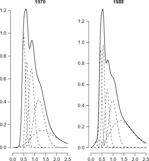
Figure 6.12 Income distribution in the United Kingdom in 1979 and 1988 (incomes normalized by contemporary mean).

z₃ for households where all the adults work, z₄ if there is no adult working in the house­hold (in a nonretired household), and z₅ for the number of children.

An ordered probit model is used to specify the relationship between the probabilities and the covariates. If a coefficient is positive (negative), then the position of an observa­tion with the associated variable moves to the right (left) of the distribution as the variable zι increases. On the other hand, a value of αι that is not significantly different from zero, indicates that the characteristic z_l does not help us to explain the decomposition of the sample into the different groups. From the results, we can see that retired (z₁) and nonworking (z₄) households are more likely to be found toward the bottom of the income distribution, and households where all adults work (z₃), on the contrary, are more likely to be found toward the right of the distribution. In addition, the position of retired households has improved over this period, whereas that of households where no one works has deteriorated. These results emphasize the usefulness of mixture models, which yield an overall picture of the distribution of income and how this has changed over time, with richer results than those obtained from other commonly employed techniques.

6.3.3.4 Finite Mixture of Regressions

Covariates have been introduced in the probabilities to characterized group profiles. They can be also introduced into the modeling of the densities in each of the groups, leading us to consider mixtures of regression models. Let us consider a mixture of Normal distributions with varianceand mean being conditional on some covariates, μ_k = xβ_k, which can be written as:

κ

If there are two groups (κ = 2), one just needs to consider the following model:

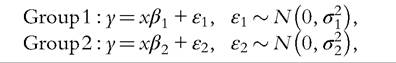
where E₁ and E₂ are independent and identical Normally distributed error terms within each group, with variances ofandrespectively. In this model, we consider that the population is composed of two different groups, for which the relationship between the dependent and explanatory variables is different, and the observations come from the dif­ferent groups in the population in unknown proportions. This specification would be particularly appropriate if we assume that the marginal impact of covariates may be dif­ferent in each of the groups, as suggested in Figure 6.3. Covariates could be introduced at the same time in the probabilities to explain group profiles.

To illustrate, consider a simple Mincer earnings equation, which explains the logarithm of an individual’s earnings by their number of years of education and number of years of labor-market experience. One way of testing for earnings differences between men and women is to test if the parameters of the earnings equation are statistically significantly dif­ferent between the two groups of individuals, via a Chow test (Chow, 1960). Table 6.4 shows ordinary least squares (OLS) estimation results from linear regression models for the groups of men and of women (columns 1 and 2), using data from a household survey carried out by the U.S. Census Bureau in May 1985.³⁰ A Chow test, equal to 14.19, rejects the null hypothesis that the two sets of coefficients are identical. As the dependent variable is the log of earnings, the estimation results show that one additional year of education increases earnings by around 7.9% for men and 10.9% for women on average. The earnings profiles as a function of labor-market experience are different between the two groups. These are traced out in Figure 6.13 for 8 years of education, from which we can see that the gender gap is sharply increasing with labor-market experience during the first 30 years.³¹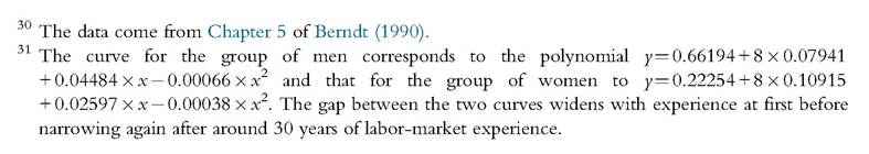

Table 6.4 Mincer earnings equations

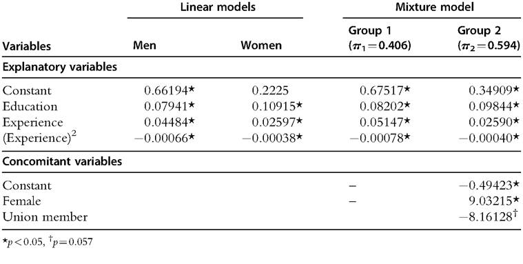
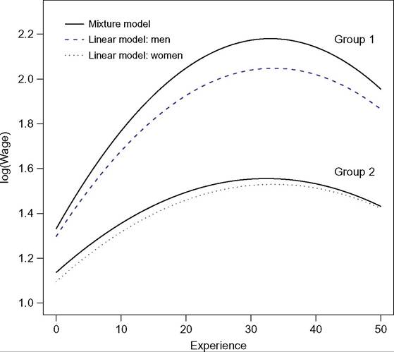
Figure 6.13 The relationship between earnings and labor-market experience.

In the linear model approach, we define a priori two groups of individuals—men and women. By contrast, in a mixture model approach, we do not specify the groups a priori, we let the data identify homogeneous groups with respect to the relationship between the dependent and explanatory variables. Table 6.4 shows estimation results from a mixture model (columns 3 and 4); the BIC suggests that there are two groups. The estimation results show that one additional year of education increases earnings by around 8.2% for individuals in the first group and 9.8% for individuals in the second, on average. The impact of experience on earnings are traced in Figure 6.13 for 8 years of education (solid lines).^[193] From this figure, the gap between the two groups is much larger than the gap between the groups of men and of women obtained from linear models.

The use of concomitant variables in the mixture model allows us to characterize the profile of the groups. Two dummy variables are taken into account as concomitant vari­ables. The first is for the individual being a woman (Female), and the second for the indi­vidual being a union member (Union Member). In Table 6.4, column 4, the positive and significant coefficient on the “Female” variable indicates that women are more likely to belong to the second group than to the first group. The negative significant coefficient on “Union Member” shows that unionized workers are less likely to belong to the second than to the first group.^[194] A classification shows that 96.3% of women belong to group 2, whereas the analogous percentage of men is only 19%.^[195] Equally, the percentage of union members classified in group 1 is 80.2%. Last, the results of this analysis suggest that, for the vast majority of women, the relationship between earnings and experience is much flatter than that for most men and union members, holding everything else equal. The gap obtained is much larger than those obtained by considering all men and all women in two distinct groups.

For more details on mixture models of regression, see McLachlan and Peel (2000), Frfihwirth-Schnatter (2006), and Ahamada and Flachaire (2010).

6.3.4 Finite Sample Properties

In this section, we study the quality of the fit of nonparametric density estimation in finite samples. To asses the quality of the density estimation, we need to use a distance measure between the estimated density and the true density. We use the mean integrated absolute errors (MIAE) measure,

1

2

1

i

1

Table 6.5 shows the quality ofthe fit for several density estimation methods. We first consider standard kernel estimator, with fixed bandwidth selected by the Silverman rule- of-thumb (Silv.), by cross-validation (CV) and by the plug-in (Plug-in) methods. Then, we consider adaptive kernel methods based on each of the previous fixed bandwidths. Finally, we consider density estimation based on mixture of lognormal distributions.³⁵

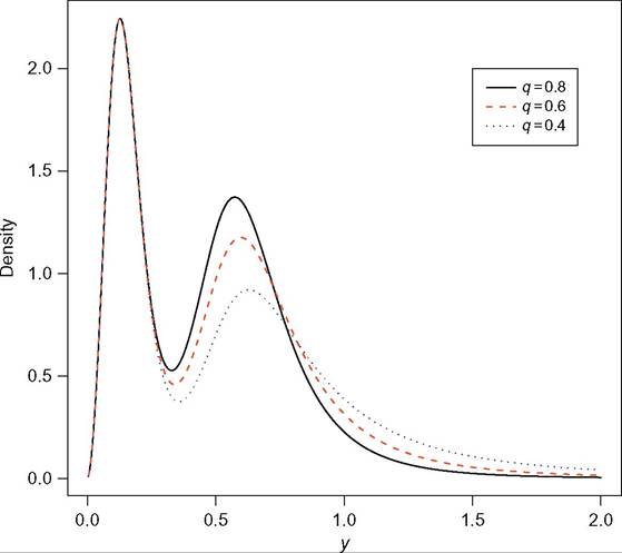
Figure 6.14 Mixture of two Singh-Maddala distributions.

³⁵ The density function of the logarithmic transformation of the data is estimated by a mixture of normal distributions and the number of components is selected with the BIC.

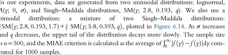
Table 6.5 Quality of density estimation (MIAE), n¼500

id="Picutre 442" class="lazyload" data-src="/files/uch_group77/uch_pgroup315/uch_uch7351/image/image441.jpg">

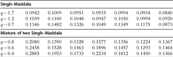
The results in Table 6.5 show that, for standard and adaptive kernel methods, the qual­ity of the fit deteriorates as the upper tail becomes heavier (as σ increases and q decreases, MIAE increases). Moreover, standard kernel method with the Silverman’s rule-of-thumb bandwidth fails when the distribution is multimodal and highly skewed (case of two Singh-Maddala distributions), compared to other methods. Finally, our results suggest that, in the cases of heavier-tailed distributions, the adaptive kernel based on the plug­in bandwidth and the mixture oflognormals perform better than standard kernel methods.

6.4.