WELFARE INDICES
We can use the term welfare indices to cover a number of specific tools of distributional analysis that are of interest to economists and social scientists. These include social welfare functions, inequality measures, and poverty indices.
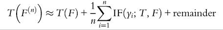
Our approach is to characterize some basic classes of indices, to introduce some standard results that enable us to describe the statistical properties of these indices, and then to apply the analysis to particular welfare indices that are of interest to students of income distribution. The applications here will be to inequality and poverty indices.6.4.1 Basic Cases
It is useful begin with two of the simplest welfare indices, the quantile and the income cumulation. Quantiles and income cumulations are themselves incomes and so belong to the interval Y = [y,y), introduced in Section 6.1.2. Once again we work with

(Gastwirth, 1971). For any distribution F the quantile functional gives the smallest income in Y such that 100q percent of the population have exactly that income or less. In cases where the distribution F is understood, we can use a shorthand form for the qth quantile
The functional Q provides the basis for several intuitive approaches to the analysis of income distribution. For example, commonly used quantile ratios — such as the “90/10” ratio, the “90/50” ratio (Alvaredo and Saez, 2009; Autoret al., 2008; Burkhauser et al., 2009)—are found by taking pairs of instances of (6.23) with appropriate q-values: y9which becomes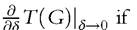 T is differentiable.
The IF is particularly useful in analyzing the problem of data contamination (see Section 6.6.1). But the IF has other convenient applications: its relevance to this part of our discussion is that it may be used to derive asymptotic results such as asymptotic covariance matrices. If the distribution G is “near” F (as in Equation (6.33) for small δ) then the first-order von Mises expansion of T at F evaluated in G is given by
When the observations are independently and identically distributed according to F then, by the Glivenko-Cantelli theorem, the empirical distribution So we may
replace G by for sufficiently large n and obtain
from which we obtain (Hampel et al., 1986, p. 85):
Lemma 1 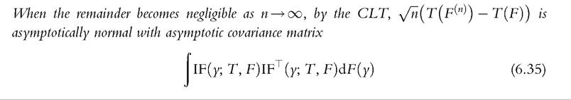
Regularity conditions can be found in Reeds (1976), Boos and Serfling (1980), and Fernholz (1983).
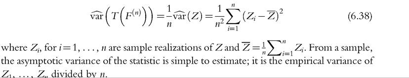
Lemma 1 constitutes the basis of the results that follow. Given a statistic T, one just needs to compute its IF to obtain the asymptotic covariance matrix. For inequality and poverty measures (unidimensional statistics), Tis a functional F → R. In many cases, we can express the IF as a random variable Z minus its expectation,
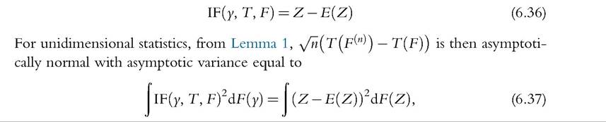
which is nothing but the variance of Z. This result allows us to estimate the asymptotic variance of the statistic from a sample using
The main issue here is to provide IFs and to express them as a function of Z as in (6.36), for a wide range of welfare indices and ranking tools, as well as for different forms of data.
Moreover, for some important cases, we will also develop analytically the formula in (6.35) so that the approach for computing asymptotic covariance matrices based on the IF can be compared to those from other approaches in the literature.386.4.2.2 Background Results
Several useful results in income distribution analysis can be found from a simple application of the IF; in particular, we have two key properties for the fundamental functionals introduced in Section 6.4.1 (Cowell and Victoria-Feser, 2002). Applying (6.23) to the distribution in (6.33), we get the qth quantile in the mixture distribution:
38 For previous suggestions on the use of the IF for estimating asymptotic variances, see, for example, Efron (1982) and Deville (1999).
where yq = Q(F, q) is the qth quantile for the (unmixed) income distribution. Letfbe the density function for the distribution function F; then, differentiating (6.39) with respect to δ and setting δ = 0, we obtain the following result.
Lemma 2
The IFfor the quantile functional is
Likewise, if we apply (6.25) to the distribution in (6.33), we get the qth income cumulation in the mixture distribution:
where Q(G, q) is given by (6.39). Once again, differentiating (6.41) with respect to δ and setting δ = 0 we obtain another basic result.
Lemma 3
The IFfor the cumulative income functional is

We will find that these results are useful not only for welfare indices considered in this section but also for distributional comparisons treated in Section 6.5.
6.4.2.3 QAD Welfare Indices
Let us first deal with the broad Wqad class, the welfare indices that are quasi-additively decomposable; we will turn to the important, but more difficult, rank-dependent class Wrd later.
Fortunately, this class covers a great number of commonly used tools of distributional analysis; fortunately also the properties are straightforward. Given a sample y1,..., yn, the sample analogues of Wqad defined in (6.30) are given by
where F(n is the EDF defined in Equation (6.8) and μ is the sample mean:
Substituting the mixture distribution (6.33) into (6.30), differentiating with respect to δ and evaluating at δ = 0, we find the IF for the QAD class as:

where φμ denotes the partial derivative with respect to the second argument. This IF can be expressed as in (6.36), that is, as a random variable Z minus its expectation,

where
6.4.3 Application: Inequality Measures
Almost all commonly used inequality indices other than the Gini coefficient can be writ broad Wqad class to derive the sampling distribution for a large range of inequality mea
sures. We consider two leading examples in Sections 6.4.3.1 and 6.4.3.2.
6.4.3.1 The Generalized Entropy Class
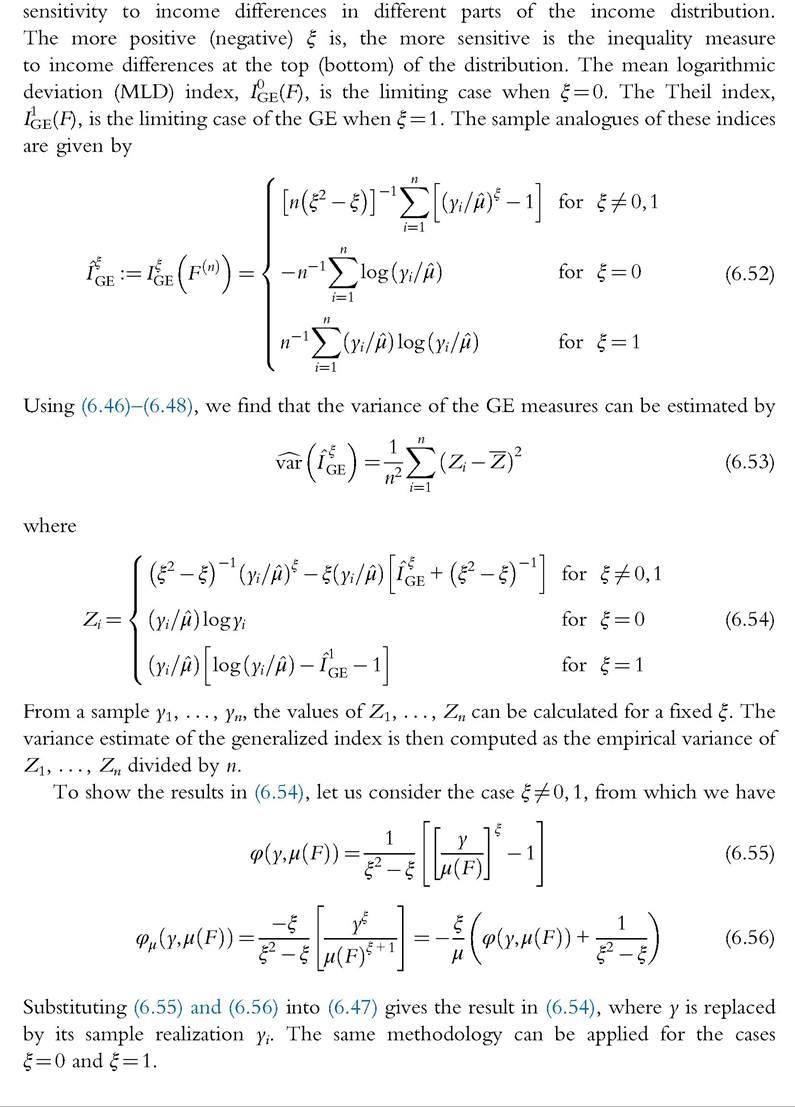
We consider first an important family of inequality measures that belongs to the additively decomposable class (6.28). Members of the GE class (characterized by the parameter ξ) are defined by Equations (6.49)-(6.51) 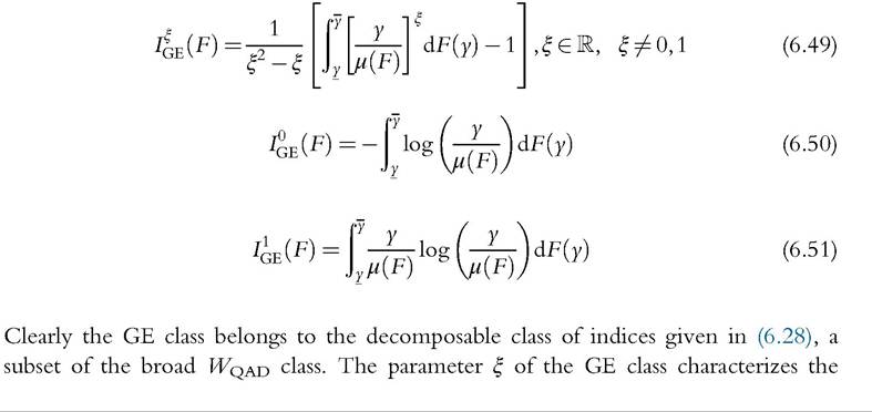
Clearly the same approach can be applied to functions of moments of the distribution such as the coefficient of variation.
Likewise, the statisticalproperties of the Atkinson class of inequality indices (Atkinson, 1970)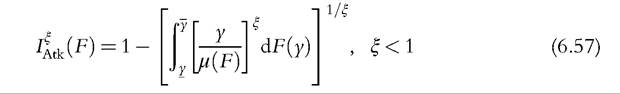
can easily be derived from (6.53).39
The standard approach to obtain the results for the GE class and associated indices is by expressing the indices as a function of moments of the distribution and using the delta method. We can show that both IF and delta approaches give the same results. Indeed, from (6.28) and (6.29), a decomposable inequality measure can written as a function of two moments,
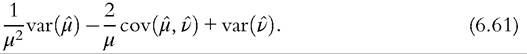
From the CLT, this estimator is also consistent and asymptotically Normal, with asymptotic variance that can be calculated by the delta method. Specifically, the asymptotic variance is equal to 
6.4.3.2 The Mean Deviation and Its Relatives
Now consider the mean deviation, an inequality index that does not belong to the class of decomposable indices (6.28), but does belong to the quasi-additive class (6.30).
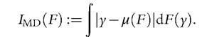
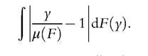
Noting that Imd(F) can be rewritten as 
40 For extensions to the case of weighted data and complex survey design, see Zheng and Cushing (2001), Cowell and Jenkins (2003), Biewen and Jenkins (2006), and Verma and Betti (2011).
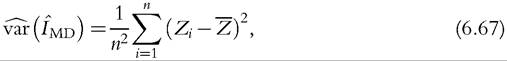
For an alternative approach to estimation of Atkinson indices using a Box-Cox transformation, see Guerrero (1987).The asymptotic variance can be estimated as the empirical variance of (Z1,..., Zn) divided by n,
where
The same methodology with some extra terms can be used to derive the asymptotic variance of the more commonly used relative mean deviation or Pietra ratio
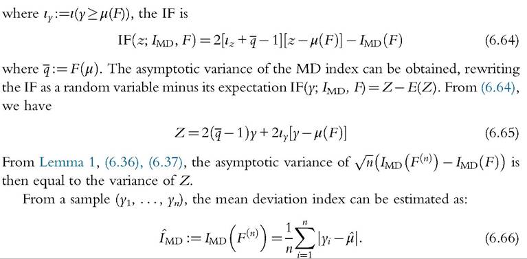
In the literature, the asymptotic variance is usually obtained with the IF method without using it expressed as a function of a random variable minus its expectation. It gives similar numerical results, but formulas and implementation are more complicated. For instance, using Lemma 1 and Equations (6.64) and (6.63), the asymptotic variance of the mean deviation can be derived as follows:
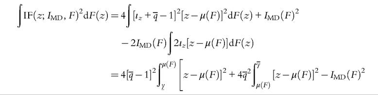
This formula for the asymptotic variance of the mean deviation index is the same as derived in Gastwirth (1974).
6.4.3.3 The Gini Coefficient
The general form (6.31) is cumbersome, but we can fairly easily derive results for the most important member of this class, namely, the Gini coefficient.
The Gini index can be expressed in a number of different forms. Let us consider the following expressions,
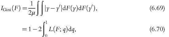
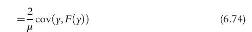
In other words, the Gini is also equal to the weighted sum of incomes using the κ weights (6.73) and is equal to 2∕μ times the covariance between y and F(y) (6.74). For the distribution-free approach, we replace μ(F) by the sample mean μ and the covariance by an unbiased estimate in (6.74). It leads us to compute the Gini index as:
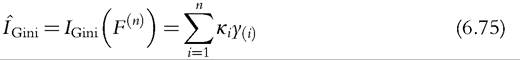
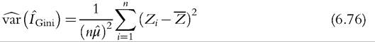
where
6.4.4 Application: Poverty Measures
For a poverty index, we need a poverty line that may be an exogenously given constant ζ or may depend on the income distribution ζ (F). An important class of poverty indices can then be described in the following way:
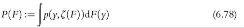
where p is a poverty evaluation function that is nonincreasing in y and takes the value zero for Ó ≥ ζ(F). Once again we need the IF, which is given by

where pζ is the differential ofp with respect to its second argument (Cowell and Victoria- Feser, 1996a). It is clear from (6.79) that the form for the asymptotic variance of the poverty index will depend on the precise way in which the poverty line depends on the income distribution. The following specifications cover almost all the versions encountered in practice

or

where yq is defined in (6.24). The interpretation is that the poverty line could be tied to the mean, as in (6.80), in which case we have
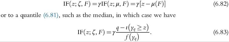
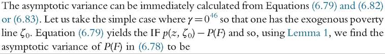
[1] Note that if γ > 0 then to estimate the asymptotic variance of P using (6.82) one needs information on the whole distribution; with (6.83) one needs a density estimate at yq.
The asymptotic variance of the poverty index is then equal to the variance of the poverty evaluation function, We can see that the preceding IF is expressed as a func
tion of a random variable minus its expectation,

From (6.36) and (6.37), the asymptotic variance is the variance of Z.
A second important class of poverty indices consists of those in the rank-dependent form—compare (6.31) above—and can be described in the following way:
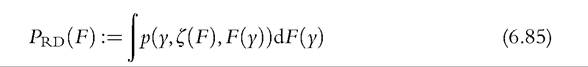
Comparing (6.85) with (6.78), we see that the poverty evaluation functionp has an extra argument reflecting the individual’s rank in the population. The IF for this class of poverty measures is more complicated (Cowell and Victoria-Feser, 1996a), and we deal with this separately in Sections 6.4.4.2 and 6.4.4.3.
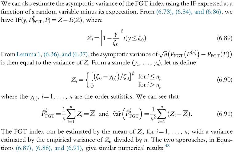
6.4.4.1 Foster-Greer-Thorbecke (FGT)
For a fixed poverty line the widely used class of poverty indices introduced by Foster et al. (1984) belongs to the class (6.78) and has the form
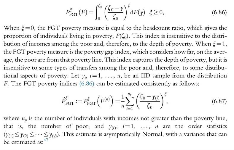
47 See Kakwani (1993).

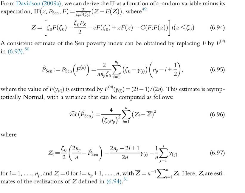
6.4.4.2 Sen Poverty Index
The Sen poverty index (Sen, 1976) belongs to the class (6.85) and can be expressed as the average of the headcount ratio and the poverty gap index, weighted by the Gini coefficient among the poor, 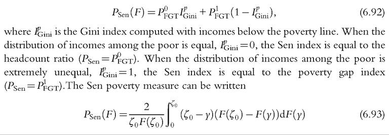
48
The problem of estimation in the presence of complex survey design is addressed in Howes and Lanjouw (1998), Zheng (2001), Berger and Skinner (2003), and Verma and Betti (2011).
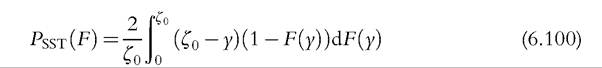
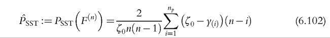
6.4.4.3 Sen-Shorrocks-Thon Poverty Index
The Sen-Shorrocks-Thon (SST) index is a convenient modified version of the Sen poverty index, defined as follows,

where is the poverty gap index computed with incomes below the poverty line, and
 is the Gini coefficient computed with individuals’ poverty gap ratios rather than individuals’ incomes for the whole population
49 In Equation (6.50) in Davidson (2009a), replacing yi in the expression of the summand by z yields the IF. The relationship to the IF is not related in the last paper; it is related in Davidson (2010), where the same method is used with S-Gini indices.
50 This expression does not coincide exactly with Sen’s own definition for a discrete population. See Appendix A in Davidson (2009a) for a discussion of this point.
51 Another variance estimator has been proposed by Bishop et al. (1997). for i = 1,..., n).52 The Gini coefficient of poverty gap ratios can be viewed as a measure of poverty inequality in a society. The SST index satisfies the transfer and continuity axioms, whereas the Sen index does not.53
This index can be decomposed into

A percentage change in SST can then be viewed as the sum of percentage changes in the proportion of poor, the average poverty gap among the poor, and one plus the Gini index ofpoverty gaps for the population. The poverty is decomposed in three aspects: Are there more poor? Are the poor poorer? Is there higher poverty inequality in the society?
The SST poverty index can be written
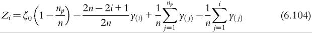
As in Section 6.4.4.2, we derive the IF as a function of a random variable minus its expec-

The SST poverty index can be consistently estimated as:55
It is asymptotically Normal, with an estimator of the variance given by
where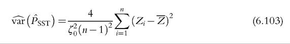

6.4.5 Finite Sample Properties
6.4.5.1 Asymptotic and Bootstrap Methods
Asymptotic Normality allows us to perform asymptotic inference. In practice, we are concerned with finite samples, and asymptotic inference can be unreliable. When asymptotic inference does not perform well in a finite sample, bootstrap methods can be used to perform accurate inference. The bootstrap appears to be an ideal method for inference with inequality and poverty indices because the observations of the sample are often IID.
Let us consider a welfare index W and its sample counterpart W. An asymptotic confidence interval at 95% would be computed as
t-statistics, that is, the ∣"0.025Bj and ∣"0.975Bj order statistics of the t*, where ∣^x^∣ denotes the smallest integer not smaller than x. In this approach, the unknown distribution of the population is replaced by the EDF of the original sample, from which we generate bootstrap samples and compute t-statistics testing the (true) hypothesis that the index is equal
56 See Beran (1988). It means that the bootstrap method presented in this section provides an asymptotic refinement over the percentile bootstrap proposed in Mills and Zandvakili (1997).
to W. The simulated distribution of the bootstrap t-statistics is used, as an approximation of the unknown distribution of t, to calculate critical values.
the samples are dependent, the statistic should take account of the covariance, and the bootstrap samples should be generated by resampling pairs of observations with replacement. Again, the bootstrap p-value would be the proportion of the τ* that is more extreme than τ.
6.4.5.2 Simulation Evidence
We now turn to the performance in a finite sample of inference based on inequality and poverty measures. The coverage rate of a confidence interval is the probability that the random interval does include, or cover, the true value of the parameter. A method of constructing confidence intervals with good finite sample properties should provide a coverage rate close to the nominal confidence level. For a confidence interval at 95%, the nominal coverage rate is equal to 95%. In this section, we use Monte Carlo simulation to approximate the coverage rate of asymptotic and bootstrap confidence intervals in several experimental designs.
In our experiments, data are generated from lognormal distributions, Λ(y; 0, σ), and from Singh-Maddala distributions, SM(y; 2.8, 0.193, q). As σ increases and q decreases the upper tail of the distribution decays more slowly. The sample size is n = 500, the number of bootstrap samples is B = 499, and the number of experiments is N = 10,000.57 When poverty indices are used, the poverty line is computed as half the median.
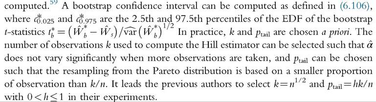
Table 6.6 presents coverage of asymptotic and bootstrap confidence intervals at the 95% level for the Theil, MLD, Gini, and SST indices. The results show that asymptotic and bootstrap confidence intervals are reliable when we consider the SST poverty index. Indeed, the coverage rates of the SST index are always close to the nominal coverage rate of 95%. In contrast, when we consider inequality measures, bootstrap confidence intervals outperform asymptotic confidence intervals, but they become less reliable as σ increases and q decreases. In other words, asymptotic and bootstrap inferences deteriorate
57
For well-known reasons—see Davison and Hinkley (1997) or Davidson and MacKinnon (2000)—the number of bootstrap resamples B should be chosen so that (B + 1)/100 is an integer.
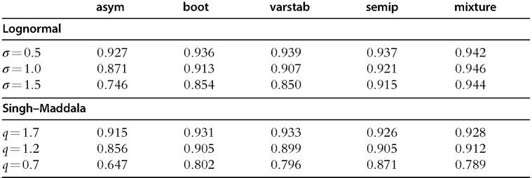
Table 6.6 Coverage of asymptotic and bootstrap confidence intervals at the 95% level for the Theil, MLD, Gini, and SST indices, n = 500
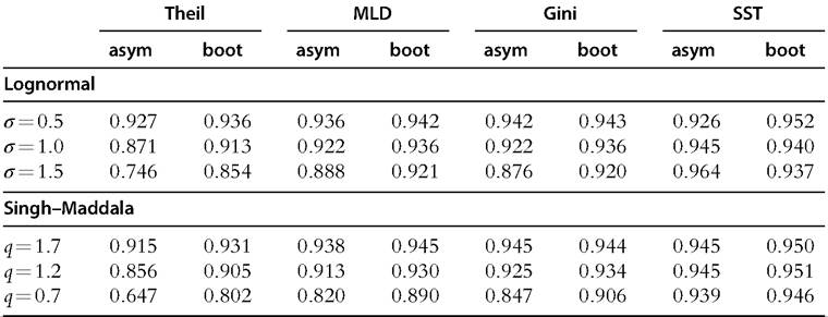
as the upper tail of the underlying distribution is heavier. For instance, asymptotic confidence intervals cover the true value of the Theil index 64.7% of times when the underlying distribution is the Singh-Maddala with q = 0.7. Bootstrap confidence intervals provide better results, with a coverage rate of 80.2%, but it is still significantly different from the expected 95%. Note that the Theil index is known to be more sensitive to the upper tail of the distribution than the MLD and Gini, and confidence intervals with the Theil index are slightly less reliable than with the MLD and Gini indices.
These results illustrate that asymptotic and bootstrap inference on inequality measures is sensitive to the exact nature of the upper tail of the income distribution. Bootstrap inference on inequality measures are expected to perform reasonably well in moderate and large samples, unless the tails are quite heavy.[198] Moreover, asymptotic and bootstrap inference on poverty measures perform well in finite samples.
6.4.5.3 Inference with Heavy-Tailed Distributions
When the distribution is one with quite a heavy upper tail, asymptotic and bootstrap inferences are known to perform poorly in finite samples. Several approaches have been proposed in the literature to obtain more reliable inference.
Schluter and van Garderen (2009) and Schluter (2012) proposed normalizing transformation of the index, before using the bootstrap, in order to use a statistic with a distribution closer to the Normal. Let g denote a transformation of the index W; a standard bootstrap confidence interval can be obtained on the transformed index g(W) and, therefore, on the untransformed index by inverting the relation between the welfare index and the parameters. be the 2.5th and 97.5 th percentiles of the EDF of the
bootstrap t-statistics
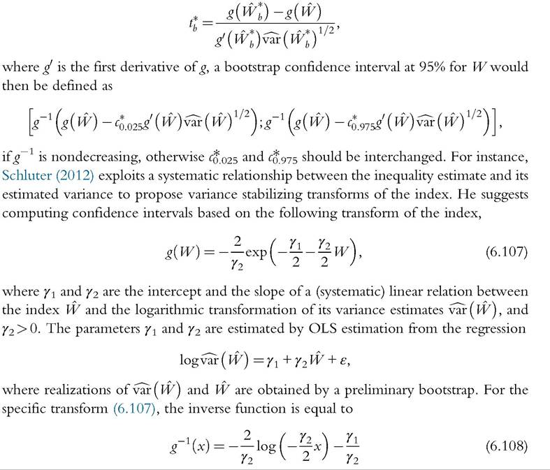
Abootstrap confidence interval at 95% can be computed using (6.107) and (6.108) in the confidence interval defined earlier.
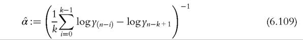
Davidson and Flachaire (2007) and Cowell and Flachaire (2007) considered a semiparametric bootstrap, where bootstrap samples are generated from a distribution that combines a parametric estimate of the upper tail with a nonparametric estimate of the rest of the distribution. The upper tail is modeled by a Pareto distribution with parameter a estimated by the Hill estimator on the k greatest order statistics of a sample of size n, for some integer k ≤ n,
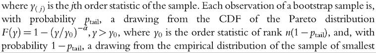
n(1 — ptail)-order statistics. For the bootstrap to test a true null hypothesis, we need to compute the value of the welfare index for the bootstrap distribution defined earlier. The CDF of the bootstrap distribution can be written as
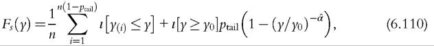
where ι(∙) is the indicator function (6.1). Indices of interests are functionals of the income distribution and so the index for this bootstrap distribution, Ws, can be
An alternative approach could be to generate bootstrap samples from a distribution estimated by finite mixture models. It allows us to estimate any density function, by allowing the number of components to vary, and, once the number of component is selected, to use a parametric distribution to generate bootstrap samples (see Section 6.3.3). For the bootstrap to test a true null hypothesis, we need to compute the value of the welfare index for the mixture distribution, Wm. With additively decomposable inequality measures, the index for the mixture distribution is easy to calculate because the mixture distribution is a decomposition by groups. For instance, the class of GE indices can be expressed as a simple additive function of within-group and between-group inequality. Let there be K groups, and let the proportion of the population falling in group k be pk, the class of GE indices is equal to60
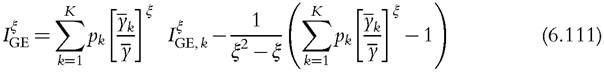
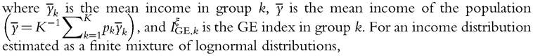
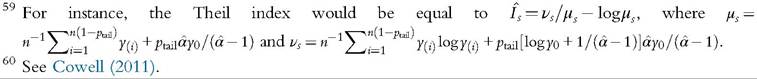
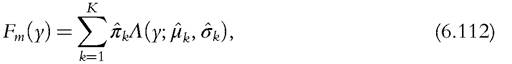
Table 6.7 presents coverage of asymptotic and bootstrap confidence intervals at the 95% level for the Theil index, with n = 500. The first two columns correspond to asymptotic (asym) and standard bootstrap (boot) methods; they reproduce the results given in Table 6.6, given here as benchmarks. The other columns show the results for the alternative bootstrap methods presented earlier. Results obtained by the approach proposed by Schluter (2012) are presented in the third column (varstab), bootstrapping a variance stabilizing transform of the Theil index. In the fourth column, the semiparametric boot-
strap proposed by Davidson and Flachaire (2007) and Cowell and Flachaire (2007) is used to generate bootstrap samples (semip), with k = n1/2 and h = 0.6. Finally, bootstrap samples generated from a mixture of lognormal distributions are considered in the last column (mixture). The simulation results show that, in the presence of very heavy-tailed distributions (σ = 1.5, q = 0.7), significant improvements can be obtained with alternative methods over asymptotic and standard bootstrap methods. However, none of the alternative methods provides very good results overall.
6.4.5.4 Testing Equality of Inequality Measures
Confidence intervals are often used to make comparisons between two or more samples. The values of an index computed from independent samples are statistically different if
Table 6.7 Coverage of asymptotic and bootstrap confidence intervals at the 95% level for the Theil index, for several bootstrap approaches, n = 500
the confidence intervals do not intersect. We can thus test if inequality or poverty measures are different between several countries, or over different periods of time, by comparing their confidence intervals. However, the previous results suggest that this approach may be unreliable when comparing inequality measures if the underlying distributions are quite heavy tailed.
Another principal way of performing inference is by carrying out hypothesis tests. Testing the equality of inequality measures with a t-statistic, Dufour et al. (2013) showed that almost exact inference can be obtained with permutation tests, if the samples come from distributions not too far away from each other, even with very heavy-tailed distributions and very small samples. They also showed that this method outperforms other methods when the distributions are far away from each other.
where τ follows asymptotically the standard Normal distribution. A standard bootstrap approach would be to generate bootstrap samples X* and Y* by resampling with replacement, respectively, n observations from X and m observations from Y. The bootstrap samples are drawings from X and Y, from which an inequality measure would provide different numerical results. The null hypothesis tested from the original sample is then not respected in the bootstrap data-generating process. A modified t-statistic has to be 546" class="lazyload" data-src="/files/uch_group77/uch_pgroup315/uch_uch7351/image/image545.jpg"> the first n and the remaining m observations of the permuted combined sample. Note that the combined sample can be permuted by resampling without replacement N observations from (X, Y).
61 Davidson and Flachaire (2007) considered testing the difference of two inequality measures with independent samples, but no significant improvement of their semiparametric bootstrap method over standard bootstrap method is found.
The permutation samples are drawings from the same set of observations; the null hypothesis tested from the original sample is then respected in the data-generating process. From a permutation sample (X*, Y*), the permutation t-statistic is
exact inference is obtained with permutation tests in very small samples with heavytailed distributions, if the samples come from distributions not too far away from each other.
portion ofp-values less than a nominal level equal to 0.05.65 Inference is exact if the rejection probability is equal to 0.05.
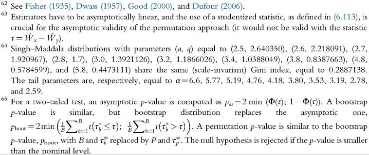
Table 6.8 Rejection frequencies of asymptotic, bootstrap, and permutation tests for testing the equality of Gini indices between two samples, when the underlying Singh-Maddala distributions are identical or different, n = 50
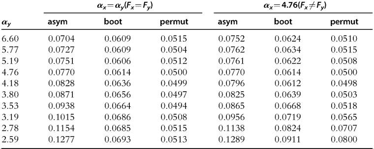
Table 6.8 shows the empirical rejection frequencies of asymptotic, bootstrap, and permutation tests for testing the equality of Gini indices between two samples, when the underlying distributions are identical and when they are different. As expected, when
Hill plots can be useful for studying the tail behavior in empirical studies. The “tail index” of a heavy-tailed distribution can be estimated by the Hill estimator on the k greatest order statistics of a sample of size n, Equation (6.109). However,
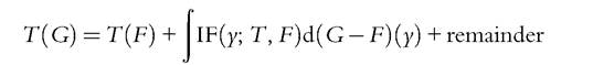
estimation results can be sensitive to the choice of k. Hill plots show the Hill estimate of the tail index as a function of the number k of the greatest order statistics used to compute it. An estimate of the tail index can be selected when the plot becomes stable about a horizontal straight line. For instance, Figure 6.15 shows Hill plots obtained from two samples of 1000 observations drawn from the Singh-Maddala distributions SM(y; 2.8, 0.193, 1.7) and SM(y; 5.8, 0.193, 0.447), with tail parameters, respectively, equal to 4.76 and 2.59, over the range 0.5% to 25% of the largest order statistic used to compute it, with 95% confidence intervals (in gray). It is clear from this figure that the second sample (right plot) comes from a much more heavy-tailed distribution than the first sample (left plot).[199]
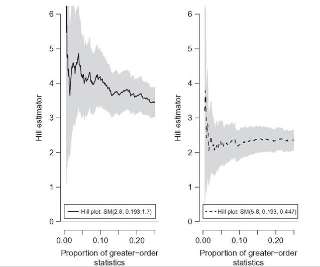
Figure 6.15 Hill plots: plot of the Hill estimate of the tail index (6.109) of two samples of 1000 observations drawn from Singh-Maddala distributions, as a function of the proportion of the greatest order statistics used to compute it.
6.4.6 Parametric Approaches
Sections 6.4.2-6.4.5 deal solely with distribution-free methods; in a sense we are working directly with the sample data. An alternative approach assumes that the distribution is known,6 up to some parameters, and can be consistently estimated. A preliminary parametric estimation of the distribution is then obtained, and the moments of the parametric distribution are estimated. When the distribution is parametric, inequality indices can be expressed as functions of the distribution parameters. Table 6.9 shows the formulas of the Theil, MLD, and GE measures of inequality for the lognormal and Pareto distributions. They are also given for the Generalized Beta distribution of the second kind (GB2), a
67 See Section 6.3.1 for a discussion of the common functional forms that may be applied.
68 SeeJenkins (2009).
derive the expressions of the Theil, MLD, and GE indices for the Singh-Maddala and Dagum distributions, set p = 1 and q = 1 in the equations given in the last column in Table 6.9. An inequality measure can be estimated by replacing the unknown parameters by consistent parameter estimates. Inequality measures are then expressed as nonlinear functions of one or several consistent estimates. From the CLT, they are asymptotically Normal, and their asymptotic variance can be derived using the delta method.[200]
For several of the standard parametric distributions, the Gini index can also be expressed fairly easily as a function of the unknown parameters of the underlying distribution. The Gini index for the lognormal distribution, , and for the Pareto dis-
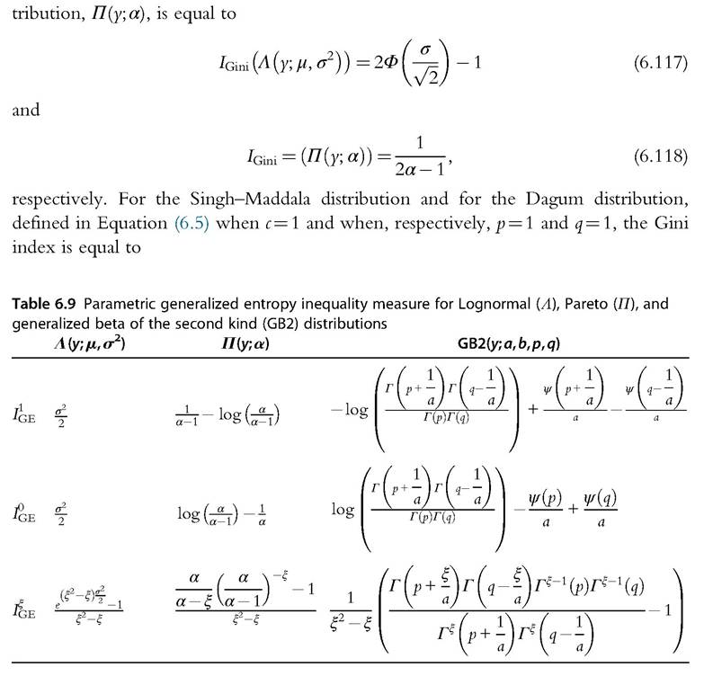
The Singh-Maddala and Dagum distributions are encompassed by the Generalized Beta distribution of the second kind (GB2), defined in Equation (6.5) when c = 1, for which the formula of the Gini index can also be obtained. However, its expression is lengthy and involves the generalized hypergeometric function, see McDonald (1984) or Kleiber and Kotz (2003) for an explicit formula. Because the Gini index is defined as nonlinear functions of one or several consistent estimates. From the CLT, it is asymptotically Normal, and the asymptotic variance can be derived using the delta method.
6.5.