DISTRIBUTIONAL COMPARISONS
Apart from the simple welfare indices discussed in Section 6.4, we also need to be able to implement ranking tools. These tools provide the researcher with intuitively appealing methods of making distributional comparisons and are associated with important results in the welfare economics of distributional analysis.
6.5.1 Ranking and Dominance: Principles
The quantile and cumulation functionals Q and C defined in Section 6.4.1 can be used to establish dominance criteria for income distribution comparisons in terms of welfare or inequality, and related concepts are available for comparisons in terms of poverty.
6.5.1.1 Dominance and Welfare Indices
6.5.1.1.1 First-OrderDominance 
To see the importance of this concept, suppose we consider the class of all indices 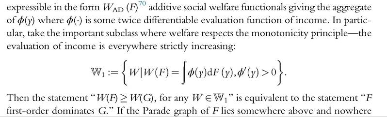 below the Parade graph of G, then welfare in F must be higher than in G, for any social welfare function that respects monotonicity (Quirk and Saposnik, 1962).
6.5.1.1.2 Second-OrderDominance
The functional (6.25) can be used to characterize a number of standard concepts associated with second-order dominance.
somewhere above and nowhere below the GLC of G, then welfare in F must be higher than in G, for any social welfare function that respects monotonicity and the transfer principle (Hadar and Russell, 1969). However, in distributional analysis attention is focused not only on the basic principle of second-order dominance, as just described, but also on restricted versions of this relationship that incorporate equivalence relationships on the members of F.
• Suppose we want the second-order comparisons to be scale independent.
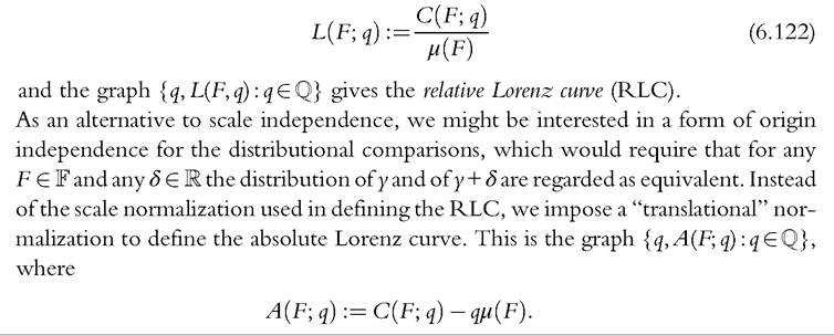
This requires that, for any and any λ > 0 the distribution of y and of y/Ë are regarded as equivalent for the purposes of distributional comparison; this implies that, when comparing distributions, we may divide incomes by an arbitrary positive constant. A natural
 70 See Equation (6.28)
choice for this constant is the mean of the distribution. The scale normalization of the GLC by the mean (6.26) gives the (relative) Lorenz functional:71
6.5.1.2 Stochastic Dominance
The first-order and second-order dominance previously defined can be encompassed in a unified method, stochastic dominance, and extended to higher-order dominance. Let us define dominance curves as follows:
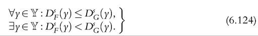
Distribution F is said to dominate distribution G stochastically at order s if the following pair of conditions holds:
The case s = 1 corresponds to first-order dominance based on Pen’s parade, previously
71 This is equivalent to the income share (6.27).
72 Fishburn (1980), O’Brien (1984), StarkandYitzhaki (1988), Thistle (1989), O’Brien and Scarsini (1991), Fishburn and Lavalle (1995), and Davidson (2008).
6.5.2 Ranking and Dominance: Implementation
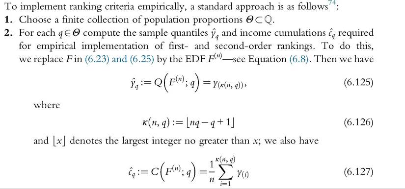
3. Compute the variances and covariances of the sample quantiles (first-order) or the income cumulations (second-order).
4. Specify carefully the ranking hypothesis that is to be tested.
Step 1—involves a choice of how many points to select on the Parade or on the Lorenz curve. Step 2 is easy. Step 3 is dealt with in Section 6.5.2.1 and Step 4 in Sections 6.5.2.3 and 6.5.2.4.
6.5.2.1 Asymptotic Distributions
The main results follow from applying Lemmas in Section 6.4.2.2. We also need to define one further functional analogous to (6.23) and (6.25):
and its sample counterpart:
73 See Atkinson (1987) and Foster and Shorrocks (1988).
74 We consider distribution-free methods. For parametric Lorenz curve comparisons, see Sarabia (2008).
Then we have the following two theorems:
Theorem 1

Proof
Immediate from Lemmas 1 and 2 ■
Theorem 2
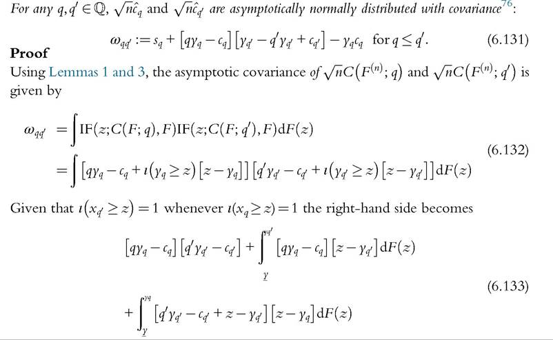
Using the definitions in (6.23), (6.25), and (6.128), we find that (6.133) becomes (6.131) ■
We can also rewrite the IF as a random variable minus its expectation. From (6.42) in Lemma 3, we have

75 See Lemma 1 of Beach and Davidson (1983).
76 See Theorem 1 of Beach and Davidson (1983).
From (6.132), we can see immediately that the asymptotic covariance of y∕ncq and y∕n^1∣ is

From a sample yi, for i = 1,..., n, we can then estimate the covariance of the GLC ordinates cq and cq' as the empirical covariance of Ziq and Ziq∕ divided by n
These results can also be used for the ordinates of the (relative) Lorenz curve.
Using the standard result on limiting distributions of differentiable functions of random variables (Rao, 1973), or using the delta method in (6.60), the asymptotic covariances of
 implementation, the components of the right-hand side of (6.139) are replaced by their sample counterparts. We can also use the IF and express it as a random variable minus its expectation. The IF of the Lorenz curve ordinate (6.122) is given by
77 Yq, Cq, and ^q are given by (6.125), (6.127), and (6.129), respectively.
78 See Cowell and Victoria-Feser (2002) and Donald et al. (2012).
Statistical Methods for DistributionalAnalysis 429
sum of IID observations, this estimator is consistent and asymptotically normal. The asymptotic covariance is also easy to calculate.79
When we compare two distributions, random samples can be obtained from two independent populations or from two correlated populations. The last case typically occurs when the two samples are independent paired drawings from the same population, as, for instance, with pretax and posttax distributions. In both cases of independent and correlated samples, it can be shown that the difference Σ)f{z^ — Dc(zq∣} is asymptotically normal, with asymptotic covariance equal to 
79
It is equal to (6.145) with F = G.
and Ds (x) estimated as defined in (6.144). For s = 2, we find an estimate of the covariance matrix similar to that obtained in (6.136) and (6.137), for the GLC ordinates. More details and explicit expressions for z being stochastic and for poverty measures can be found in the comprehensive approach to inference on stochastic dominance presented in Davidson and Duclos (2000).80
6.5.2.2 Dominance: An Intuitive Application
Armed with Theorems 1 and 2, an intuitive approach to dominance can be immediately applied.
Using (6.127) we can plot an empirical GLC with confidence bands. Consistent estimates of the variance of the GLC ordinates can be calculated using (6.136) and (6.137)
GLC for distribution F lies above that for distribution G (second-order dominance). Clearly the same idea could be pursued with empirical quantiles and parade diagrams (first-order dominance).
Figure 6.16a, to the left, shows two GLCs obtained from two independent samples of 5000 observations drawn from Singh-Maddala distributions F and G, respectively, with confidence bands at 95% evaluated at the percentiles, q = 0.01, 0.02,..., 0.99. F is the Singh-Maddala distribution with parameters a = 2.8, b = 0.193, and q = 1.7, used in the introduction, and G is the distribution with parameters a = 3.8, 0.193, and 0.839; the means are, respectively, 0.169 and 0.240. This figure shows that distribution G second-order dominates distribution F. It suggests that poverty measures based on poverty gaps will exhibit more poverty in F than in G (Jenkins and Lambert, 1997). Table 6.10 shows poverty measures computed from the two samples, with 95% confidence intervals (see Section 6.4.4). As expected, poverty indices are significantly greater in F than in G.
80 On dominance with complex sample design, see Beach and Kaliski (1986) and Zheng (1999, 2002). Foran alternative approach focusing on crossings in the tails ofLorenz curves, see Schluter and Trede (2002), and for a Bayesian approach, see Hasegawa and Kozumi (2003). On the extension to absolute dominance and deprivation dominance, see Bishop et al. (1988) and Xu and Osberg (1998), and on poverty dominance see also Chen and Duclos (2008) and Thuysbaert (2008).
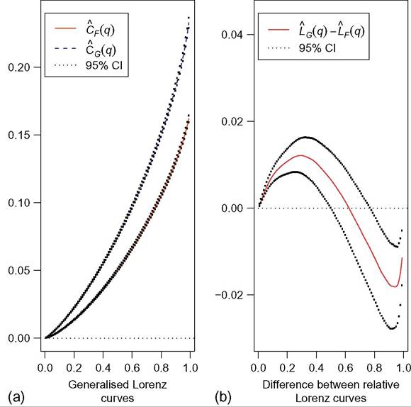
Figure 6.16 Generalized Lorenz curves and difference between Lorenz curves, n ¼ 5000.
intersect, and in such cases no unambiguous ranking can be obtained. Nevertheless, useful information on inequality can be drawn from Lorenz curve comparisons.
Figure 6.16b, to the right, shows the difference between two RLCs obtained from the two samples used in Figure 6.16a. The two curves intersect in the upper part. This figure also shows that the empirical Lorenz curve of G lies significantly above the empirical Lorenz curve of F in the bottom part, whereas the reverse is true in the upper part. It suggests that inequality measures sensitive to the bottom part of income distributions would be smaller in G than in F, whereas inequality measures more sensitive to the upper part ofincome distributions would be smaller in F than in G. Table 6.10 shows inequality measures computed from the two samples, with 95% confidence intervals (see Section 6.4.3) Noting that GE measures, ⅛e, are more sensitive to the bottom (top) of income distributions with smaller (higher) parameter ξ, we find the results suggested by the previous Lorenz curve comparisons. Indeed, IGe is significantly smaller in G than in F, whereas I^Ge is significantly smaller in F than in G.
This approach is clearly ad hoc, and we need to examine the issues involved more carefully; we do this in Sections 6.5.2.3 and 6.5.2.4. Graphical representation of two
Table 6.10 Inequality and poverty measures, with confidence intervals at 95%, computed from two samples of 5000 observations drawn independently from F and G
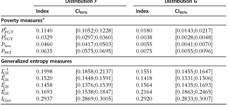
aThe poverty line is half the median of the sample drawn from distribution F: ζ0 = 0.07517397.
empirical Lorenz curves, with confidence intervals, allows us to make individual comparisons. We can test if particular Lorenz curve ordinates are significantly different between two curves. To be able to make conclusions on dominance or nondominance, we need to test simultaneously that all ordinates from one curve are significantly greater or not smaller than the ordinates from the other curve. Appropriate test statistics need to be used to make multiple comparisons and to test simultaneously that several inequalities hold. Moreover, Lorenz curve ordinates are typically strongly positively correlated and, thus, test statistics need to take into account the covariance structure between the Lorenz curve ordinates.
6.5.2.3 The Null Hypothesis: Dominance or Nondominance
Performing inference on stochastic dominance is more complex than on a single welfare index. The hypotheses tested are usually based on a set of inequalities. For instance, first- order stochastic dominance requires that,

to say that distribution F dominates distribution G stochastically at order one. The theoretical literature also include the condition that F(y) < G(y) for some y, as defined in (6.124). However, no statistical test can distinguish between these two forms of weak and strict dominance.[201] Because we are interested in statistical issues hereafter, we make no distinction between weak and strict dominance, and we can write all inequalities as weak.
Inference on dominance in the population would be drawn from the corresponding sample properties. From a given sample, we can consistently estimate the two distributions by their EDF counterparts, F(n) (x) and . Sample dominance is then defined as
  for all y. It is clear that dominance in the population cannot be rejected if there is dominance in the sample. It is rejected if sample nondominance is statistically significant only. A similar reasoning applies for nondominance in the population. It follows that, to infer dominance, we should test the null hypothesis of nondominance, and to infer nondominance, we should test the null of dominance.
It can be illustrated with a simple example of two distributions with the same sup- 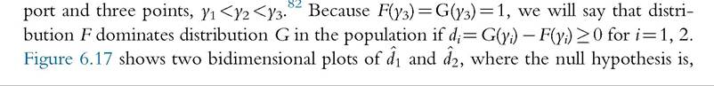
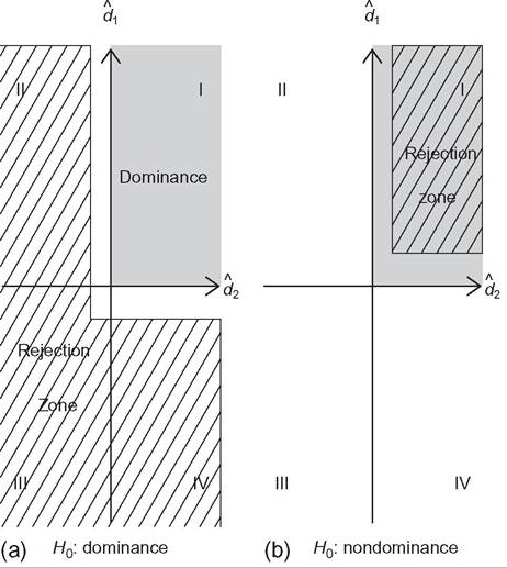
Figure 6.17 Tests of dominance and nondominance. The first quadrant, I, corresponds to dominance of G by F in the sample (gray area). The quadrants II, III, and IV correspond to nondominance.
82
See Davidson and Duclos (2013).
respectively, dominance and nondominance. Distribution F dominates G in the sample when di > 0, for i = 1, 2. Then, the first quadrant, denoted I (gray area), corresponds to dominance in the sample, whereas quadrants II, III, and IV correspond to nondominance in the sample.
First, let us consider the null hypothesis of dominance, as shown in Figure 6.17a, on the left. To reject dominance in the population, the nondominance in the sample must be statistically significant, that is, the rejection zone has to be far enough from the dominance area, for example, in the cross-hatched area. The rejection zone is exclusively in the area of nondominance, whereas the (remaining) nonrejection zone corresponds to the dominance area plus the white L-shaped band within the nondominance area. Then, rejecting the null hypothesis of dominance corresponds to the case of nondominance, whereas nonrejecting it is inconclusive.
Second, let us consider the null hypothesis of nondominance, as shown in Figure 6.17b, on the right. With a similar reasoning, we can see that the rejection zone is exclusively in the area of dominance, whereas the nonrejection zone is composed of both nondominance and dominance situations (gray L-shaped band). Then, rejecting the null hypothesis of nondominance corresponds to the case of dominance, whereas nonrejecting it is inconclusive.
The previous example illustrates that positing the null of nondominance is the only way to draw a strong conclusion of dominance. However, it comes at a cost: Dominance will be inferred only if there is strong evidence in its favor. From Figure 6.17b, we can see that rejecting the null of nondominance is quite demanding because it requires that both statistics d1 and d2 are statistically significant. It may be too demanding, especially in the tails where both distributions tend to the same values and where we usually have sparse data and little information. Davidson and Duclos (2013) showed that, with distributions continuous in the tails, it is impossible to reject the null of nondominance over the full support of the distributions. It leads them to develop restricted stochastic dominance, limiting attention to some interval in the middle of the distribution.
The most common approach in the literature has developed tests of stochastic dominance positing the null of dominance.[202] The previous example illustrates the standard feature in statistics that nonrejecting the null does not imply that the null is true, and so selecting the null hypothesis remains allows for the possibility of being wrong at some level.[203] The level at which we may be wrong by accepting the null is unknown (the L-shaped bands in Figure 6.17a and b), but it would be reduced by using statistical tests with greater power properties in a finite sample.
Finally, the two approaches can be seen as complementary. Rejecting the null of dominance or nondominance allows us to infer, respectively, nondominance and dominance when comparing two distributions.
6.5.2.4 Hypothesis Testing
Test statistics have been developed in the literature under the null hypothesis of dominance and nondominance. We distinguish both cases, for which we can interpret them, respectively, as union-intersection and intersection-union tests.
Under the Null of Dominance
Statistical tests can be constructed to test the null hypothesis of dominance against the alternative of nondominance. Under the null hypothesis that F dominates G, we have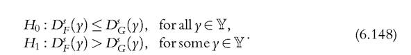
where Y denotes a given set contained in the union of the support of the two distributions. An appropriate test statistic could be interpreted as a union-intersection test because the null hypothesis is expressed as an intersection of individual hypotheses and the alternative as an union (Roy, 1953). A natural test is based on the supremum of individual differences,

It is clear that the null hypothesis is rejected if τ is significant and positive. McFadden (1989) proposed a test based on (6.149) for two independent samples of IID observations. For s = 1, it is a variant of the Kolmogorov-Smirnovstatistic, with known properties. For s = 2, the asymptotic distribution under the null is not tractable. Barrett and Donald (2003) proposed simulation-based methods for estimating critical values, taking into account comparisons at all points of the support (functional approach) rather than at a fixed number of arbitrarily chosen points. Linton et al. (2005) proposed to use subsam- 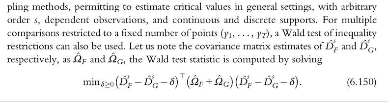
The statistic is obtained by using an algorithm to solve quadratic programming problems. The distribution of the statistic is a mixture of chi-square with weights that require simulation methods to be consistently estimated (Dardanoni and Forcina, 1999).
Lorenz dominance can be tested using similar methods. Bishop et al. (1989) and Davidson and Duclos (1997) proposed a test for a fixed number of points,85 whereas Donald and Barrett (2004) and Bhattacharya (2007) have considered versions of Lorenz dominance tests in a functional approach, taking into account comparisons at all points of the supports.
Under the Null of Nondominance
Other statistical tests have been developed to test the null hypothesis of nondominance against the alternative of dominance. Under the null that F does not dominate G, we have 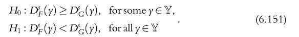 An appropriate test could be interpreted as an intersection-union test because the null hypothesis is expressed as an union and the alternative as an intersection of individual hypotheses (Gleser, 1973). The idea behind the intersection-union method is that the null is rejected only if each of the individual hypotheses can be rejected. A natural test is based on the infimum of individual differences,

It is clear that the null hypothesis is rejected if τ0 is significant and positive. The statistic τ0 has to be defined over Yr, some closed interval contained in the interior of the joint support of the two distributions Y. The main reason is that the null hypothesis would never be rejected if we consider the tails of the distributions, where data are sparse and where the differences between the two distributions tend to zero. Specifically, Yr should be a restricted interval in Y that removes the tails of the distributions. Kaur et al. (1994) proposed a test based on (6.152) for s = 2 with independent samples and continuous distributions F and G. Critical values can be taken from the Normal distribution, making the test easy to implement. However, it can have low power properties (Dardanoni and Forcina, 1999). Davidson and Duclos (2013) and Davidson (2009b) proposed a test for higher order, for correlated samples as well as uncorrelated samples, and for continuous and discrete distributions. They also showed that appropriate bootstrap methods permit researchers to obtain much better finite sample properties.
85
See also Bishop et al. (1991a,b, 1992).
6.6.
More on the topic DISTRIBUTIONAL COMPARISONS:
- Contents
- Atkinson Anthony, Bourguignon François. Handbook of Income Distribution. Volume 2A. North Holland,2014. — 2366 p., 2014
- The Meaning of Welfarism and Non-welfarism
- CHOOSING A YARDSTICK AND ITS COMPONENTS
- THE COMPARATIVE VIEW
- CONCLUSION
- REFERENCES