OTHER ESTIMATION PROBLEMS

In Sections 6.4 and 6.5, we assumed that data are always drawn from a representative sam­ple of the whole population. For some researchers this state of affairs is something of a luxury.

6.6.1 Contamination

By data contamination we mean a set of observations that do not “belong” to the sample—see Section 6.2.3. The essentials of the formal approach can be explained using a simple model based on the distribution function (in fact, we have already seen the ele­ments of this model in a different context—see Section 6.4.2). The idea is that, instead of observing a distribution F 2 F directly, one sees it after it has been mixed with another distribution that represents contamination. The elementary model of this is presented in Equation (6.33), where one observes a distribution G given by

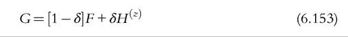
where δ represents the proportion of contamination in the mixture that we observe and H(^z) is the elementary “contamination distribution” (6.32), a single point mass at z 2 Y. From this minimalist structure, one can easily develop more interesting specifications of the model of contamination using a mixture of F with a distribution that is richer than H(^z). A number of questions immediately arise: Does contamination matter in analyzing income distributions? How does contamination affect distributional comparisons? How may one appropriately estimate models of income distribution if there is reason to believe that contamination is an important issue?

6.6.1.1 The Concept of Robustness

To address the question “how important,” we can use the tool introduced in the dis­cussion of asymptotic inference (Section 6.4.2).

6.6.1.2 Robustness, Welfare Indices, and Distributional Comparisons

Does contamination matter for the tools that we discussed in Sections 6.4 and 6.5?

Basic cases. First, take two statistics whose properties can be easily deduced, the mean and median. Using the definition of the mixture distribution (6.153) with point­contamination (6.32) and the linearity of the mean functional, we can write the mean of the observed mixture distribution as

Evaluating (6.154) for the elementary point-contamination distribution (6.32), we obtain

The observed mean is a simple weighted sum (with weights 1 — δ, δ) of the true mean μ(F) and the value of z where the contamination is concentrated.

It is easy to see from (6.156) that IF(z; μ, F) is unbounded as z tends to -∞ or +∞: The mean is a nonrobust statistic. So if you want to use the mean as a welfare index, then the introduction of a very small amount of contamination sufficiently far out in one of the tails of the distribution will cause the observed value of the mean to be pulled away from the true value.⁸⁶ Now consider the median, as a particular case of the quantile func­tional (6.23); using the basic result Lemma 2 and setting q = 0.5 to obtain the median we have

⁸⁶ Using (6.42), the same type of reasoning can be used to show that Lorenz ordinates are also nonrobust (Cowell and Victoria-Feser, 2002).

It is clear that, as long as there is positive density at the median y₀.₅, the IF in (6.157) is bounded (Cowell and Victoria-Feser, 2002). So, in contrast to the mean, the median is robust. The intuition is clear: if you throw a single alien observation into the formula for the mean then, if that observation is large enough, it can have a huge effect when aver­aged in with the other sample values. But the median simply marks the “halfway” point in the distribution: If you introduce a single alien observation to the right of the median, then the size of that observation (how far it is to the right of the median) has no effect on the observed halfway point.

Inequality. It turns out that most commonly used inequality indices behave in a way that is similar to the mean: they are nonrobust (Cowell and Victoria-Feser, 1996b). To see why, let us check the properties of the WQ_ad class of welfare indices (6.30) on which many standard inequality measures are based.

where φ(y, μ(F)) is the evaluation of each individual income y used in the formula (6.30). It is clear that contamination could have an impact through more than one route—there is the direct effect from the evaluation of z, the first term in (6.158); there is also an indirect route through the effect on the mean, the third term in (6.158). Notice that this indirect route contains the expression, z — μ(F), as the right-hand side of (6.156). From this we can see that if φ_μ(z,μ(F)) is not everywhere zero, contamination will cause quasi-additive welfare indices to be nonrobust. Now consider the direct route: Clearly if φ(z,μ(F)) is unbounded as z approaches infinity or as z approaches zero, the particular index in the Wq_ad class will be nonrobust; this is precisely what happens with nearly all commonly used inequality measures.^[204] Why does this happen? Inequality measures are usually designed to be sensitive to extreme values at one or other end of the distri­bution, so placing a tiny amount of contamination sufficiently far out in one of the tails is going to have a big impact on measured inequality because of its built-in sensitivity. As an example, take the GE measures. From Equations (6.49)-(6.51) we see that

of top-sensitive members of the GE family and for contamination near zero in the case of bottom-sensitive members of the GE family.^[205]

Poverty. By contrast, conventional poverty indices such as the FGT class (6.86) and the Sen index (6.93) are robust if the poverty line is exogenous or is a function of a robust statistic such as the median (Cowell and Victoria-Feser, 1996a).

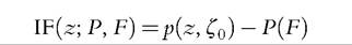
where p(∙) is the poverty evaluation function. From (6.86), we can see that for the FGT class

language contamination at the very bottom of the distribution (below the poverty line) has an impact that it is bounded below, but a very high observation has no effect on pov­erty, whether that observation is a genuine high income or contamination. Poverty mea­sures such as the FGT class are robust under contamination.

6.6.1.3 Model Estimation

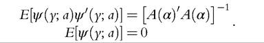
If inequality measures are typically nonrobust, what is to be done about the possibility of contamination? A potentially useful approach is to use a parametric functional formf(y;^) to model all or part of the income distribution and then compute inequality from the modeled distribution. But of course the robustness property of the inequality index based on the modeled distribution will depend on the way the parameter vector θ 2 R^p is estimated. If one consider using maximum likelihood estimators (MLEs), for example, the robustness problem remains. Although MLEs are attractive in terms of their efficiency properties, they are usually nonrobust. If we consider the wider class of M-estimators characterized by^[206]

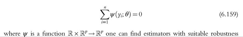
properties. These are the bounded-IF M-estimators with minimal asymptotic covariance matrix, known as Optimal Bias-Robust Estimators (OBRE)—see Huber (1981) and

Hampel et al. (1986). One can see OBRE as the solution to a trade-off between efficiency and robustness.

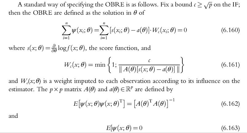
The constant c acts as a regulator between efficiency (high values of c) and robustness (low values of c).

6.6.2 Incomplete Data

We now turn to the problems of estimation and inference in a situation where, in part of the sample, some information is unavailable. As we noted in Section 6.2.3, this situation is sometimes imposed by data providers, sometimes created by researchers who are attempting to deal with problems of data contamination as discussed in Section 6.6.1.

6.6.2.1 Censored and Truncated Data

Here, we are dealing with the cases summarized in the first row of Table 6.2 in Section 6.2.3 in which we take z and z as fixed boundaries.

Truncated data. For data represented by Case A in Table 6.2, inference can be approached as for inference in the complete-information case with a redefined popula­tion: The limits ofthe support ofthe distribution (y, y) are replaced by the narrower trun­cation limits (z, z). If we wish to say more, it may be possible to use a parametric method to estimate the truncated part of the distribution.

Censoring with minimal information. Now consider Case B in Table 6.2. Clearly if we do not use the observed point masses at z and z, this could be just treated as Case A.

90

See Victoria-Feser and Ronchetti (1994), Cowell and Victoria-Feser (1996b), and for grouped data, see Victoria-Feser and Ronchetti (1997).

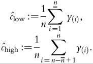
However, if we want to do more, first-order comparisons can be carried out. We need the following statistics: n (the full sample size), n (the number of observations equal to z), and n (the number of observations equal to z).

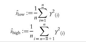
Censoring with rich information. Clearly it is possible to do more in Case C than in the previous two cases: More welfare indices (for the whole population) can be handled. Depending on the richness of information in the censored parts, it may be possible to carry out inference on Lorenz curve ordinates and some welfare indices. First, if, in addi­tion to the information described in the discussion of Case B, the means of the censored parts of the sample are given,⁹¹ then second-order rankings and the Gini coefficient can be estimated. Then it makes sense to define the following:

Inference may also be possible using the same methodology as for the complete data case. To do this, we would additionally need the following information

If these variance terms from the excluded portion of the sample are also made available, then the asymptotic variances and covariances for the income cumulations (GLC ordi­nates) forare found as follows. Replace (6.127) and (6.129) by the following

and plug into (6.138). To compute asymptotic variance for the (relative) Lorenz curve and the Gini coefficient, we also need the following:

91

In some cases means will be available from data providers.

Comparing the outcome from these computations with the full-information case in Section 6.5.2.1, we can draw two important conclusions (Cowell and Victoria-Feser, 2003). First, if the necessary information about the censored part of the distribution is used, the standard errors are the same as in the full information case. Second, when the information about the censored part is not available, the standard errors are smaller.

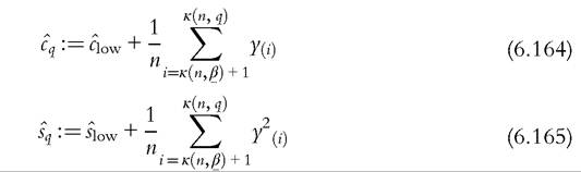
6.6.2.2 Trimmed Data

In the case of trimmed data, a fixed proportion of the sample is discarded—see the second row of Table 6.2. The trimmed samples for computing welfare indices and making dis­tributional comparisons are usually based on robustness arguments (Cowell and Victoria- Feser, 2006): outliers may seriously bias the point estimates as well as the variances of the distributional statistics that are of interest—see the discussion in Section 6.6.1.

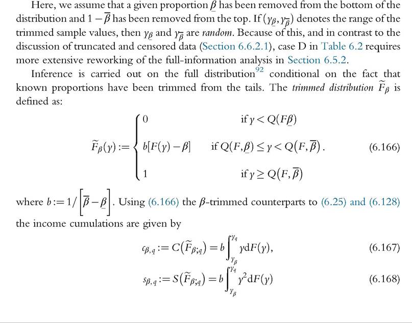
⁹² Given that the integration of IF. IF^t is required over the full distribution to derive the asymptotic covari­ance matrix, this might appear to invalidate the applicability of nonparametric techniques because of the lack of information on the structure of the trimmed data. Cowell and Victoria-Feser (2003) show that this supposition is groundless.

and then we may compare the results with those in the complete-information case.⁹⁴ Using the definition of the IF then (6.171) implies that IF for the cumulative income functional with trimmed data is⁹⁵

Compare this with (6.139).

QAD Welfare indices. To evaluate inequality and poverty indices we can again follow the method of Section 6.4, but perform the computations on the trimmed distribution Fβ defined in (6.166)—once again ignoring the information on the excluded part of the sample. This means that the trimmed version of (6.30) becomes

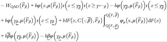
which is the counterpart of (6.43) but applied to the trimmed sample. Evaluating the IF we have⁹⁶

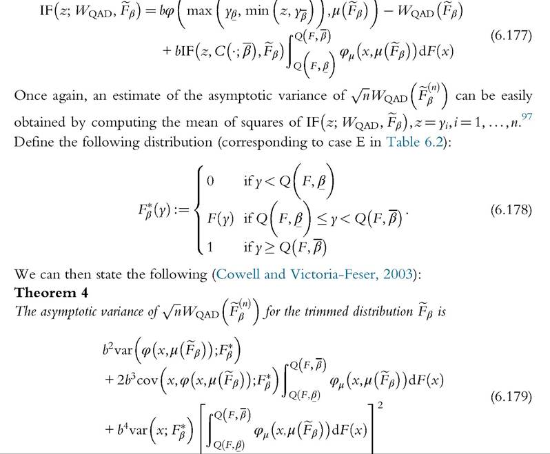
Note that in (6.179) the variance and covariance terms for the linear functionals are defined on the distribution F* as opposed to the trimmed distribution (6.166). All the components of (6.179) can be estimated from the trimmed sample.

^[1] To see this evaluate the mixture distribution and apply (6.34) to get

The Gini coefficient. With trimmed data, the Gini coefficient can be expressed as

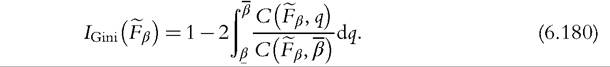
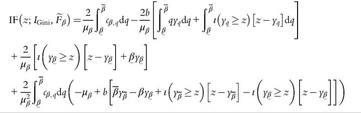
Using the same procedure as before, we first evaluate the IF for the Gini coefficient with trimmed data as:

6.6.3 Semiparametric Methods

The problems that we address here may have arisen from situations where the researcher has concerns about data contamination and robustness (see Section 6.6.1) or where the data provider has truncated or censored the data (see Section 6.6.2).

The type of problem to be analyzed can be simplified if we restrict attention to one leading case. If the support of the income distribution is bounded below, then the prob­lems with contaminated data are going to occur only in the upper tail of the distribution (Cowell and Victoria-Feser, 2002). It may be reasonable to use a parametric model for the upper tail of the distribution (modeled on a proportion β 2 Q of upper incomes) and to use the EDF directly for the rest of the distribution (the remaining proportion the 1 — β of lower incomes). There are four main issues:

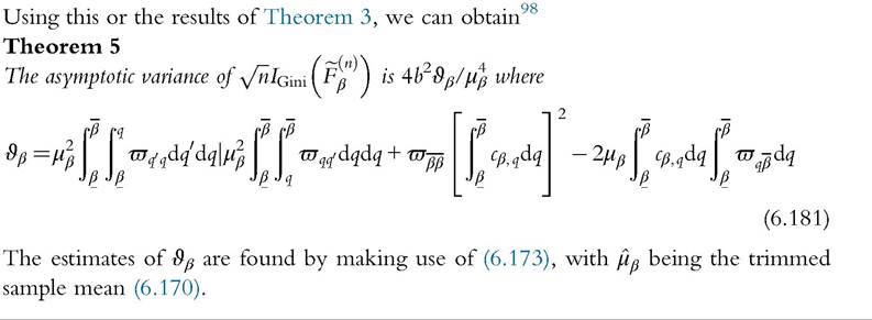
^[1] For proof of IF (z; IGi_ni, -^eβ) and Theorem 5 see Cowell and Victoria-Feser (2003).

^[1] This section draws on Cowell and Victoria-Feser (2007).

• What parametric model should be used for the tail?

• How should the model be estimated?

• How should the proportion β be chosen?

• What are the implications for welfare indices and dominance criteria?

6.6.3.1 TheModel

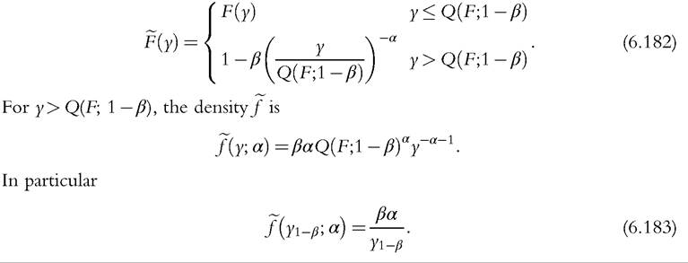
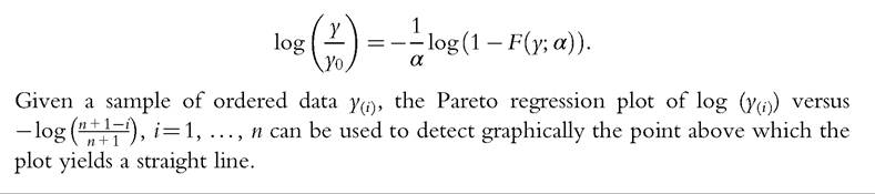
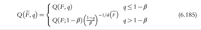
The parametric model most commonly used for the upper tail is the Pareto distribution (6.2)—see the discussion in Section 6.3.1.1. In principle the Pareto model has two parameters: We suppose here that the parameter y₀ is determined by the 1 — β quantile Q(F; 1 — β) defined in (6.23); the dispersion parameter α is of special of interest and is to be estimated from the data.^[207]

The semiparametric distribution is then

6.6.3.2 Model Estimation

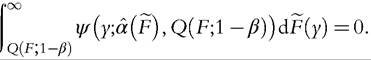
To estimate the Pareto model for the upper tail of the distribution, one could of course use the MLE but the MLE for the Pareto model is known to be sensitive to data con­tamination (Victoria-Feser and Ronchetti, 1994). Alternatively one could use OBRE as discussed in Section 6.6.1.3, with p = 1. Given a sample {y_i, i = 1,..., n} and a bound c ≥ 1 on the IF, the OBRE are defined implicitly by the solution ^F) in

100

with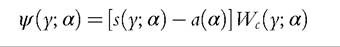

A(α) and vector a(α) are defined implicitly by

As explained in Section 6.6.1.3, the constant c parameterizes the efficiency-robustness trade-off.A common method for choosing c is to choose an efficiency level (relative to that of MLE) and derive the corresponding value for c: for the Pareto model, a value of c = 2 leads to an OBRE achieving approximately 85% efficiency.

6.6.3.3 Choice of β

Clearly one could adopt a heuristic approach selecting by eye the amount β of the upper tail to be replaced.

Alternatively one could use the robust approach in Dupuis and Victoria-Feser (2006), who develop a robust prediction error criterion by viewing the Pareto model as a regres­sion model. Rearranging (6.2) or (6.4), one can represent the linear relationship between the log of the y and the log of the inverse CDF:

6.6.3.4 Inequality and Dominance

The effect on inequality of semiparametric modeling is easy to see. For example, if we wish to see how the GE indices are affected, one substitutes F—defined in (6.182)—into (6.49)-(6.51) to obtain. For first-order and second-order dominance results, we need to look once more at the quantile and cumulative income functionals.

The quantile functional obtained using (6.182) is given by

The cumulative income functional becomes

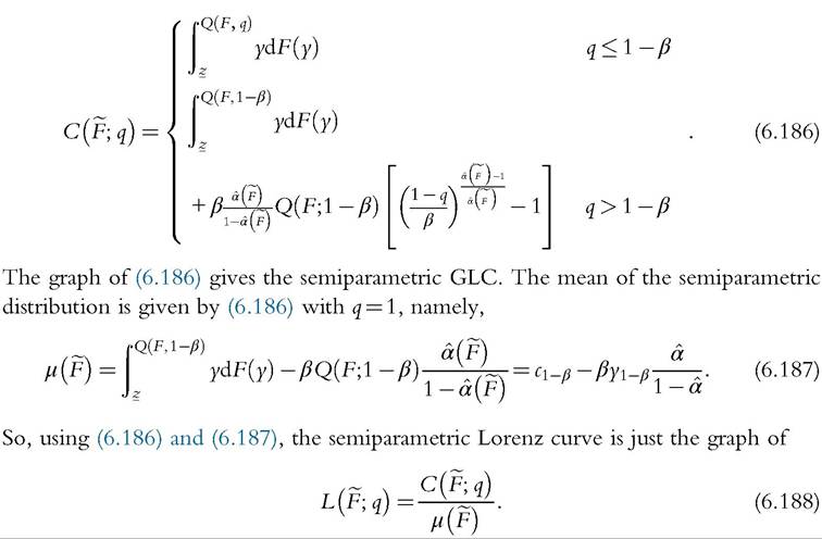
Estimates of the GLC and the Lorenz curve for the semiparametric model can be found by replacing F with F⁽ⁿ⁾ in (6.182) to obtain

¹⁰¹ The data are from the Luxembourg Wealth Study, a harmonized database that facilitates international comparisons—see http://www.lisdatacenter.org/our-data/lws-database/. See Cowell (2013) for more detail of this example.

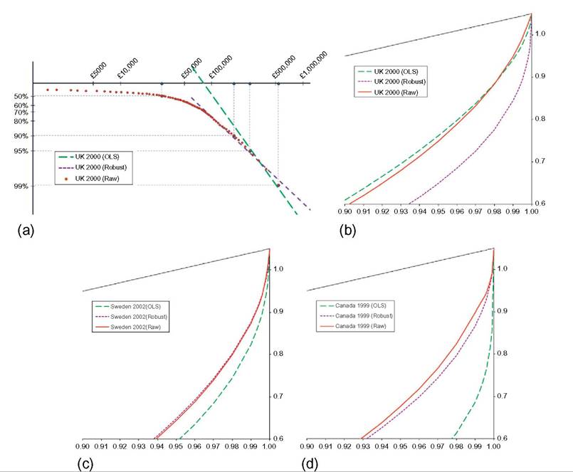
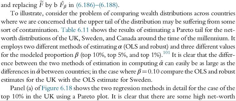
Figure 6.18 Semiparametric modeled Lorenz curves of net worth.

observations that “pull down” the OLS regression line so to speak; if one down-weights these observations, as in the robust regression, one finds a much flatter regression line, corresponding to a lower value of α and, consequently, a higher estimate of inequality within the top 10% group. The results of OLS and robust methods used in semipara­metric modeling are further illustrated for this case in Figure 6.18b, which shows the Lorenz curves for the raw data and for the semiparametric distributions produced by OLS and robust regression. Notice that if one considers the robust method appropriate, then the Lorenz curve for the whole distribution will lie well outside the Lorenz curve for the raw data and for the OLS semiparametric distribution.

Notice that the contrast between the OLS and robust estimates can differ dramatically between countries. This is evident from a comparison of the UK with Sweden or with Canada in Table 6.11. In the case of Sweden and Canada, the outliers pull the regression line in the opposite direction from that seen in the case of the UK: The robustly

Table 611 Estimates of a for net worth usinα different Snecifications of b

Source: LuxembourgWealth Study.

Table 6.12 Estimates of the Gini coefficient for net worth from raw data and from semiparametric distributions

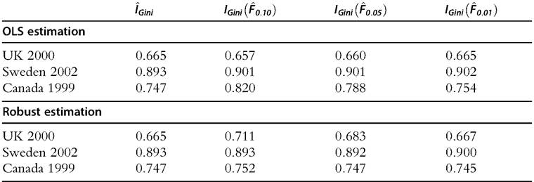
Source: LuxembourgWealth Study.

computed α is accordingly higher than that found under OLS. The consequence for the Lorenz curves is shown in Figure 6.18c and d; it is clear that for Sweden and Canada the robustly estimated semiparametric Lorenz curve is close to the Lorenz curve for the raw data, but the OLS-estimated Lorenz curve is quite far away.

The effect of the different estimation methods on inequality within the top 100β% is obvious—remember that the Gini coefficient for a Pareto distribution with parameter α is just 1Z[2α — 1]. The resulting effect on Gini in the whole distribution is shown in Table 6.12. Although the effect can be quite large for β = 0.10, in none of the cases modeled here does it change the conclusion about the ranking by inequality of the three countries.

6.7.