Descriptive Analysis of Changes over Time
A strong motivation for computing multidimensional poverty is to track and analyse changes over time. Most data available to study changes over time are repeated cross-sectional data, which compare the characteristics of representative samples drawn at different periods with sampling errors, but do not track specific individuals across time.
This section describes howto compare M0 and its associated sub-indices over time with repeated cross-sectional data. It offers a standard methodology of computing such changes, and an array of small examples. This section does not treat the data issues underlying poverty comparisons, and readers are expected to know standard techniques that are required for such rigorous empirical comparisons. For example, the definition of indicators, cutoffs, weights, etc. must be strictly harmonized for meaningful comparisons across time, which always requires close verification of survey questions and response structures, and may require amending or dropping indicators. The sample designs of the surveys must be such that they can be meaningfully compared, and basic issues like the representativeness and structure of the data must be thoroughly understood and respected. We presume this background in what follows. This section focuses on changes across two time periods; naturally the comparisons can be easily extended across more than two time periods.9.2.1 CHANGES IN M0, H, AND A ACROSS TWO TIME PERIODS
The basic component of poverty comparisons is the absolute pace of change across periods.[233] The absolute rate of change is the difference in levels between two periods.
Changes (increases or decreases) in poverty across two time periods can also be reported as a relative rate. The relative rate of change is the difference in levels across two periods as a percentage of the initial period.
For example, if the M0 has gone down from 0.5 to 0.4 between two consecutive years, then the absolute rate of change is (0.5 - 0.4) = 0.1. It tells us how much the level of poverty (M0) has changed: 10% of the total possible set of deprivations that poor people in that society could have experienced has been eradicated; 40% remains. The relative rate of change is (0.5 - 0.4)/0.5 = 20%, which tells us that M0 has gone down by 20% with respect to the initial level. While absolute changes are fundamentally important and easy to understand and compare, both absolute and relative rates may be important to report and analyse. The value-added of the relative changes is evident in relatively low-poverty regions. A region or country with a high initial level of poverty may be able to reduce poverty in absolute terms much more than one having a low initial level of poverty. It is, however, possible that although a region or country with low initial poverty levels did not show a large absolute reduction, the reduction was large relative to its initial level and thus it should not be discounted for its slower absolute reduction.[234] The analysis of both absolute and relative changes gives a clear sense of overall progress.
The relative rate of change (δ) is the difference in Adjusted Headcount Ratios as a percentage of the initial poverty level and is computed for M0, H, and A (only M0
shown) as

If one is interested in comparing changes over time for the same reference period, the expressions (9.8) and (9.11) are appropriate. However, in cross-country exercises, one may often be interested in comparing the rates of poverty reduction across countries that have different periods of reference. For example the reference period of one country may be five years, whereas the reference period for another country is three years.
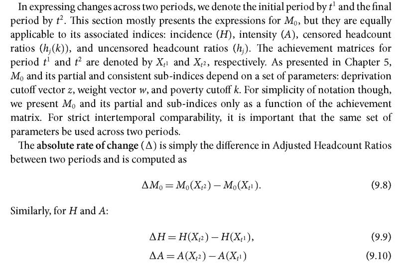
It is evident in Table 9.2 that the reference period of Nepal is five years (2006-11), whereas that of Peru is only three years (2005-8). In such cases, it is essential to annualize the change in order to preserve strict comparison.The annualized absolute rate of change (Δ) is the difference in Adjusted Headcount Ratios between two periods divided by the difference in the two time periods (t2 — t1) and is computed for M0 as
The annualized relative rate of change (δ) is the compound rate of reduction in M0 per year between the initial and the final periods, and is computed for M0 as
As formula (9.8) has been used to compute the changes in H and A using formulae (9.9) and (9.10), formulae (9.11) to (9.13) can be used to compute and report annualized changes in the other partial and consistent sub-indices, namely H, A, hj(k), or hj.
9.2.2 AN EXAMPLE: CHANGES IN THE GLOBAL MPI
Table 9.2 presents both the annualized absolute and annualized relative rates of change in global MPI, as outlined in Chapter 5, and its two partial indices—H and A—for four countries: Nepal, Peru, Rwanda, and Senegal, drawing from Alkire, Roche, and Vaz (2014). Taking the survey design into account, we also present the standard errors (in parentheses) and the levels of statistical significance of the rates of reduction, as described in the Appendix of Chapter 8. The figures in the first four columns present the values and standard errors for M0, H, and A in both time periods. The results show that Peru had the lowest MPI with 0.085 in the initial year, while Rwanda had the highest with 0.460.
Table 9.2 Reduction in MPI, H, and A in Nepal, Peru, Rwanda, and Senegal
Notes: *** statistically significant at ω = 0.01, ** statistically significant at ω = 0.05, * statistically significant at ω = 0.10.
These figures have been computed so as to be strictly comparable with harmonized indicator definitions, and therefore do not match the MPI values released in UNDP reports.Source: Alkire, Roche, and Vaz (2014)
Under the heading ‘Annualized Change', Table 9.2 provides the annualized absolute and annualized relative reduction for M0, H, and A, which are computed using equations (9.12) and (9.13). It shows, for example, that Nepal, with a much lower initial poverty level than Rwanda, has experienced a greater absolute annualized poverty reduction of -0.027. In relative terms, Nepal outperformed Rwanda. Peru had a low initial poverty level, and reduced it in absolute terms by only -0.006 per year, which means that the share of all possible deprivations among poor people that were removed was less than one-fourth that of Nepal or Rwanda. But relative to its initial level of poverty, its progress was second only to Nepal. It is thus important to report both absolute and relative changes and to understand their interpretation. The same results for H and A are provided in Panels II and III of the table. We see that Nepal reduced the percentage of people who were poor by 4.1 percentage points per year—for example, if the first year 64.7% of people were poor, the next year it would be 60.6%. Peru cut the poverty incidence by 1.3 percentage points per year. Relative to their starting levels, they had similar relative rates of reduction of the headcount ratio. Note that when estimates are reported in percentages, the absolute changes are reported in ‘percentage points' and not in ‘percentages'. Thus, Nepal's reduction in H from 64.7% to 44.2% is equivalent to an annualized absolute reduction of 4.1 percentage points and an annualized relative reduction of 6.3%.
Table 9.3 Changes in the number of poor accounting for population growth
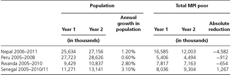
Note: Population figures correspond to United Nations, Department of Economic and Social Affairs, Population Division (2013), World Population Prospects: The 2012 Revision, DVD Edition.
Figures for Senegal 2010/11 correspond to the average between both years.Source: Authors' presentation, based on Alkire, Roche, and Vaz (2014)
The third column provides the results for the hypothesis tests which assess if the reduction between both years is statistically significant.[235] The reductions in M0 in Nepal and Rwanda are significant at ω = 0.01, but the same in Peru is only significant at ω = 0.10. Interestingly, the reduction in intensity of poverty in Peru is significant at ω = 0.05. The case of Senegal is different in that the small reduction in M0 is not even significantly different at ω = 0.10, preventing the null hypothesis that the poverty level in both years remained unchanged from being rejected.
9.2.3 POPULATION GROWTH AND CHANGE IN THE NUMBER OF Multidimensionallypoor
Besides comparing the rate of reduction in M0, H, and A as in Table 9.2, one should also examine whether the number of poor people is decreasing over time. It may be possible that the population growth is large enough to offset the rate of poverty reduction. Table 9.3 uses the same four countries as Table 9.2 but adds demographic information. Nepal had an annual population growth of 1.2% between 2006 and 2011, moving from 25.6 to 27.2 million people, and reduced the headcount ratio from 64.7% to 44.2%. This means that Nepal reduced the absolute number of poor by 4.6 million between 2006 and 2011.
In order to reduce the absolute number of poor people, the rate of reduction in the headcount ratio needs to be faster than the population growth. The largest reduction in the number of multidimensionally poor has taken place in Nepal. A moderate reduction in the number of poor has taken place in Peru and Rwanda. In contrast, there has been an increase in the total number of multidimensionally poor in Senegal, from 8 million to over 9 million between 2005 and 2011.
9.2.4 DIMENSIONAL CHANGES (UNCENSORED AND CENSORED HEADCOUNT RATIOS)
The reductions in M0, H, or A can be broken down to reveal which dimensions have been responsible for the change in poverty.
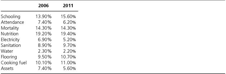
This can be seen by looking at changes in the uncensored headcount ratios (hj) and censored headcount ratios (hj(k)) described in section 5.5.3. We present the uncensored and censored headcount ratios of MPI indicators for Nepal in Table 9.4 for years 2006 and 2011 and analyse their changes over time. For definitions of indicators and their deprivation cutoffs, see section 5.6. Panel I gives levels and changes in uncensored headcount ratios, i.e. the percentage of people that are deprived in each indicator irrespective of deprivations in other indicators. Panel II provides levels and changes in the censored headcount ratios, i.e. the percentage of people who are multidimensionally poor and simultaneously deprived in each indicator. By definition, the uncensored headcount ratio of an indicator is equal to or higher than the censored headcount of that indicator. The standard errors are reported in parentheses.As we can see in the table, Nepal made statistically significant reductions in all indicators in terms of both uncensored and censored headcount ratios. The larger reductions in censored headcount are observed in electricity, assets, cooking fuel, flooring, and sanitation; all censored headcount ratios have decreased by more than 3 percentage points. Nutrition, mortality, schooling, and attendance follow with annual reductions of 3,2.3,1.8, and 1.5 percentage points, respectively.
The changes in censored headcount ratios depict changes in deprivations among the poor. Recall that the overall M0 is the weighted sum of censored headcount ratios of the indicators as presented in equation (5.9) and the contribution of each indicator to the M0 can be computed by equation (5.10). Because of this relationship, the absolute rate of reduction in M0 in equation (9.8) and the annualized absolute rate of reduction in M0 in equation (9.12) can be expressed as weighted averages of the absolute rate of reductions in censored headcount ratios and annualized absolute rate of reductions in censored headcount ratios, respectively. When different indicators are assigned different weights, the effects of their changes on the change in M0 reflect these weights.[236] For example, in the MPI, the nutrition indicator is assigned three times more weight than electricity. This implies that a one percentage point reduction in nutrition ceteris paribus would lead to an absolute reduction in M0 that is three times larger than a one percentage point reduction in the electricity indicator.
Recall that it is straightforward to compute the contribution of each indicator to M0 using its weighted censored headcount ratio as given in equation (5.10). Note that interpreting the real on-the-ground contribution of each indicator to the change in M0 is not so mechanical. Why? A reduction in the censored headcount ratio of an indicator is not independent of the changes in other indicators. It is possible that the reduction in the censored headcount ratio of a certain indicator j occurred because a poor person
Table 9.4 Uncensored and censored headcount ratios of the global MPI, Nepal 2006-1 1
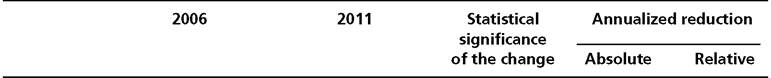
Panel I: Uncensored Headcount Ratio
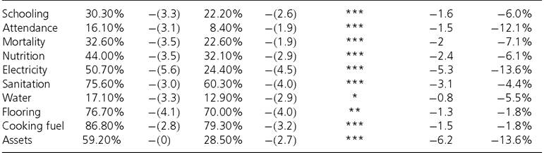
Panel II: Censored Headcount Ratio
Panel III: Dimensional Contribution to MPI
Note: *** statistically significant at ω = 0.01, ** statistically significant at ω = 0.05, * statistically significant at ω = 0.10 Source: Alkire, Roche, and Vaz (2014)
became non-deprived in indicator j. But it is also possible that the reduction occurred because a person who had been deprived in j became non-poor due to reductions in other indicators, even though they remain deprived in j. In the second period, their deprivation in j is now censored because they are non-poor (their deprivation score does not exceed k). The comparison between the uncensored and censored headcount distinguishes these situations. For example, we can see from Panel I of Table 9.4 that the reductions in the uncensored headcount ratios of flooring and cooking fuel are lower than the annualized reductions of the censored headcount ratios of the these two indicators. Thus some non-poor people are deprived in these indicators. In intertemporal analysis it is useful to compare the corresponding censored and uncensored headcount ratios to analyse the relation between the dimensional changes among the poor and the society-wide changes in deprivations. Of course in repeated cross-sectional data, this comparison will also be affected by migration and demographic shifts as well as changes in the deprivation profiles of the non-poor.
Panel III of Table 9.5 presents the contribution of the indicators to the M0 for Nepal in 2006 and in 2011. The contributions of assets, electricity, and attendance have gone down, whereas the contributions of flooring, cooking fuel, sanitation, and schooling have gone up. The contributions of water, nutrition and mortality have not shown large changes. Dimensional analyses are vital and motivating because any real reduction in a dimensional deprivation of the poor will certainly reduce M0. Real reductions are normally those which are visible both in raw and censored headcounts.14
9.2.5 SUBGROUP DECOMPOSITION OF CHANGE IN POVERTY
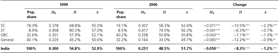
subgroup f, as in equation (5.7). It is extremely useful to analyse poverty changes by population subgroups, to see if the poorest subgroups reduced poverty faster than less poor subgroups and to see the dimensional composition of reduction across subgroups (Alkire and Seth 2013b, 2015; Alkire and Roche 2013; Alkire, Roche, and Vaz 2014). Population shares for each time period must be analysed alongside subgroup trends. For example, let us decompose the Indian population into four caste categories: Scheduled Castes (SC), Scheduled Tribes (ST), Other Backward Classes (OBC), and the General category. As Table 9.5 shows, M0 as well as H have gone down statistically significantly at the national level and across all four subgroups, which is good news. However, the reduction was slowest among STs who were the poorest as a group in 1999, and their intensity showed no significant decrease. Thus, the poorest subgroup registered the slowest progress in terms of reducing poverty.
To supplement the above analysis it is useful to explore the contribution of population subgroups to the overall reduction in poverty, which not only depends on the changes in subgroups' poverty but also on changes in the population composition. This can be seen
14 Comparisons of reductions in both raw and censored headcounts may be supplemented by information on migration, demographic shifts, or exogenous shocks, for example.
Table 9.5 Decomposition of M0, H, and A across castes in India
Note: *** statistically significant at ω = 0.01, ** statistically significant at ω = 0.05, * statistically significant at ω = 0.10 Source: Alkire and Seth (2013b, 2015)
Note that the overall change depends both on the changes in subgroup M0,s and the changes in population shares of the subgroups.
9.3