Changes over Time by Dynamic Subgroups
The overall changes in M0, H, and A discussed thus far could have been generated in many ways. It might be desirable for policy purposes to monitor how poverty changed.
In particular, one may wish to pinpoint the extent to which poverty reduction occurred due to people leaving poverty vs a reduction of intensity among those who remained poor, and also to know the precise dimensional changes which drove each.For example, a decrease in the headcount ratio by 10% could have been generated by an exit of 10% of the population who had been poor in the first period. Alternatively, it could have been generated by a 20% decrease in the population who had been poor, accompanied by an influx of 10% of the population who became newly poor. Furthermore, the people who exited poverty could have had high deprivation scores in the first period—that is, been among the poorest—or they could have been only barely poor. The deprivation scores of those entering and leaving poverty will affect the overall change in intensity (ΔA) as will changes among those who stay poor. In addition, these entries into and exits from poverty could have been precipitated by different possible increases or decreases in the dimensional deprivations people experienced in the first period, which will then be reflected in the changes in uncensored and censored headcount ratios.
This section introduces more precisely these dynamics of change. We first show what can be captured with panel data, then show empirical strategies to address this situation with repeated cross-sectional data. Finally we present two approaches related to Shapley decompositions which appear to decompose changes precisely, but rely on some crucial assumptions so their empirical accuracy is questionable.
9.3.4 EXITS, ENTRIES, AND THE ONGOING POOR: A TWO-PERIOD PANEL
Let us consider a fixed set of population of size n across two periods, t1 and t2.
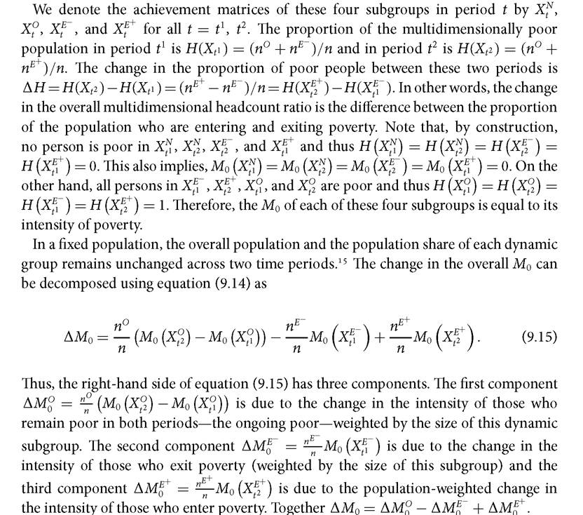
The achievement matrices of these periods are denoted by Xt1 and Xt2. The population can be mutually exclusively and collectively exhaustively categorized into four groups that we refer to as dynamic subgroups, as follows:Subgroup N Contains nN people who are non-poor in both periods t1 and t2
Subgroup O Contains n0 people who are poor in both periods t1 and t2 (ongoingpoor) Subgroup E- Contains nE people who are poor in period t1 but exit poverty in period t2 Subgroup E+ Contains nE+ people who are not poor in period t1 but enter poverty in period t2
From this point there are many interesting possible avenues for analyses. Each group can be studied separately or in different combinations. For policy, it could be interesting to know who exited poverty and their intensity in the previous period, to see if the poorest of the poor moved out of poverty. The intensity of those who entered poverty shows whether they dipped into the barely poor group or catapulted into high-intensity poverty, perhaps due to some shock or crisis or (if the population is not fixed) migration. Intensity changes among the ongoing poor show whether their deprivations are declining, even though they have not yet exited poverty. Dimensional analyses of changes for each dynamic subgroup, which are not covered in this book but are straightforward extensions of this material, are also both illuminating and policy relevant.
In the case of panel data with a fixed population we are able to estimate these precisely. We can thus monitor the extent to which the change in M0 is due to movement into
15 Suitable adjustments can be made for demographic shifts when the population is not fixed across two periods.
and out of poverty, and the extent to which it is due to a change in intensity among the ongoing poor population. The example in Box 9.1 may clarify.
BOX 9.1 DECOMPOSING THE CHANGE IN M ACROSS DYNAMIC SUBGROUPS: AN ILLUSTRATION
Consider the following six-person, six-dimension g0 matrices, in which people enter and exit poverty, and intensity among the poor also increases and decreases.
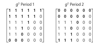
Let us use a poverty cutoff of 33% or two out of six dimensions. Increases and decreases are depicted in bold.
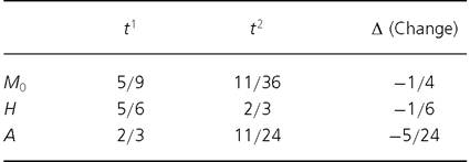
Below we summarize M0, H, and A in two periods and their changes across two periods.
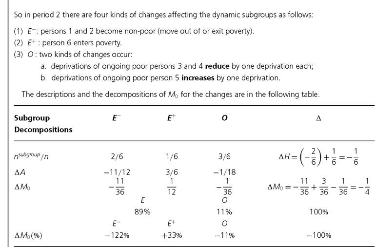
BOX 9.1 (cont.)
What is particularly interesting for policy is that we can notice that, in this example, 11% of the reduction in poverty was due to changes in intensity among the 50% of the population who stayed poor, that poverty was effectively increased 33% by the new entrant, but that this was more than compensated by those who exited poverty (-122%), because they initially had very high intensities. In this dramatic example, the poorest of the poor exited poverty, while the less poor experienced smaller reductions.
9.3.2 DECOMPOSITION BY INCIDENCE AND INTENSITY FOR CROSS-SECTIONAL DATA
The previous section explained the changes for a fixed population over time. To estimate that empirically requires panel data with data on the same persons in both periods which can be used to track their movement in and out of poverty. Yet analyses over time are often based on repeated cross-sectional data, having independent samples that are statistically representative of the population under study, but that do not to track each specific observation over time. This section examines the decomposition of changes in M0 for cross-sectional data.
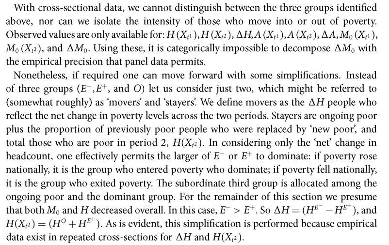
Example: Suppose that 37% of people are ongoing poor, 3% enter poverty, 13% exit poverty, and 47% remain non-poor. Suppose the overall headcount ratio decreased by 10 percentage points, and the headcount ratio in period 2 is 40%, whereas in period 1 it was 50% (37%+13%). We now primarily consider two numbers: the headcount ratio in period 2 of 40% (interpreted broadly as ongoing poverty) and the change in headcount ratio of 10% (interpreted broadly as moving into/out of poverty). In doing so we are effectively permitting the ‘new poverty entrants' to be considered as among the group in ongoing poverty in period 2 (37% + 3% = 40%). To balance this, we effectively replace 3% of those who exited poverty (13% — 3% = 10% = ΔH), and consider this slightly reduced group to be those who moved out of poverty. If poverty had increased overall, the swaps would be in the other direction.
16 The corresponding considerations apply if poverty has increased and He is expected to be small.
17 Naturally it is also possible to create estimates for A0 where the upper bound was the overall change in intensity, and the lower bound was zero, and solve for Ae. However this would not permit an increase in intensity (which would happen if the barely poor left poverty and the others stayed the same, for example), nor for an even stronger reduction in intensity. For example, in the example in Table 9.2, Nepal’s A reduced by five percentage points, whereas in our upper bound, intensity among the stayers increased by 4% and in the lower bound it decreased by 13%.
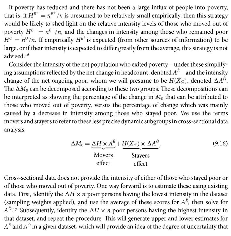
different assumptions introduce. To estimate stricter upper and lower bounds it could be assumed that those who moved out of poverty had an intensity score of the value of k (the theoretically minimum possible), and subsequently assume that their intensity was 100% (the theoretically maximum possible).[237]
Table 9.6 provides the empirical estimations for the upper and lower bounds for the same four countries discussed above plus Ethiopia.
At the upper bound, those who moved out of poverty could have had average intensities ranging from 59% in Peru (the least poor country) to 99% in Ethiopia or 100% in Senegal, according to the datasets. This in itself is interesting, as it would suggest that Rwanda—the poorest country of the four—had movers with lower average deprivations than Ethiopia. Those who stayed poor would have had, in this case, small if any increases or decreases in intensity—less than four percentage points. At the lower bound, those who moved out of poverty could have had intensities from 33% in Peru and Senegal to 38% in Nepal, and intensity reductions among the ongoing poor could have ranged from 2% in Senegal to 13% in Nepal. At the upper bound (where we assume the poorest of the poor moved out of poverty), for Nepal, Rwanda, and Peru, over 100% of the poverty reduction was due to the movers, because intensity among the ongoing poor would have had to increase (to create the observed ΔM0)∙ At the lower bound, where the least poor people moved out of poverty, movers contributed 47-67% to ΔM0. Senegal did not have a statistically significant reduction in poverty. Ethiopia provides a different example where the upper and lower bounds are closer together and reductions in intensity among the ongoing poor would have contributed 31% to 73%.This empirical investigation shows that, when implemented with the mild assumptions that are required for cross-sectional data, the upper and lower bounds according to each country's dataset are very wide apart. In reality, the relative contribution of the movers and stayers to overall poverty reduction could vary anywhere in this range.
As the example shows, the empirical upper and lower bounds vary greatly across countries. In the case of Ethiopia, movers explain 27% to 69% of the changes in poverty, and stayers account for 31% to 73%. These boundaries do not permit us to assess whether the actual contribution from movers was greater than or less than that of stayers.
In Nepal and Peru the movers probably contributed more than stayers to poverty reduction, as in all cases their lowest effect is above 50%. Given these wide-ranging upper and lower bounds, empirically we are unable to answer questions such as whether the intensity of the ongoing poor decreased, or whether it was the barely poor or the deeply poor who moved out of poverty. While this can seem disappointing, for policy purposes, as Sen stresses, it may be better to be ‘vaguely right than precisely wrong', and repeated cross-sectional data simply do not permit us, at this time, to move ahead with precision.Table 9.6 Decomposing the change in M0 by dynamic subgroups
| Panel A | ||||||||||
| Country | M | colspan=4 bgcolor=white>HA | AH | |||||||
| t1 | t2 | AM0 | t1 | t2 | t1 | t2 | ||||
| Ethiopia 2005-2011 | 0.605 | 0.523 | -0.081 | 89.7 | 84.1 | 67.4 | 62.3 | 5.66 | ||
| Nepal 2006-2011 | 0.350 | 0.217 | -0.133 | 64.7 | 44.2 | 54.0 | 49.0 | 20.55 | ||
| Peru 2005-2008 | 0.085 | 0.066 | -0.019 | 19.5 | 15.7 | 43.6 | 42.2 | 3.78 | ||
| Rwanda 2005-2010 | 0.460 | 0.330 | -0.130 | 82.9 | 66.1 | 55.5 | 49.9 | 16.75 | ||
| Senegal 2005-2010/1 1 | 0.440 | 0.423 | -0.017 | 71.3 | 70.8 | 61.7 | 59.7 | 0.46 | ||
Panel B
Shapley
Country Upper bound Lower bound decomposition
| A Movers | AA Stayers | Movers' effect | Stayers' effect | A Movers | AA Stayers | Movers' effect | Stayers' effect | Incidence effect H | Intensity effect A | |
| Ethiopia 2005-201 1 | 0.99 | -0.03 | 68.7% | 31.3% | 0.38 | -0.07 | 26.6% | 73.4% | 45% | 55% |
| Nepal 2006-201 1 | 0.74 | 0.04 | 113.4% | -13.4% | 0.38 | -0.13 | 58.2% | 41.8% | 79% | 21% |
| Peru 2005-2008 | 0.59 | 0.02 | 119.5% | -19.5% | 0.33 | -0.04 | 67.1% | 32.9% | 86% | 14% |
| Rwanda 2005-2010 | 0.78 | 0 | 101.4% | -1.4% | 0.36 | -0.1 | 47.1% | 52.9% | 68% | 32% |
| Senegal 2005-2010/11 | 1 | -0.02 | 26.8% | 73.2% | 0.33 | -0.02 | 8.9% | 91.1% | 16% | 84% |
9.3.3 THEORETICAL INCIDENCE-INTENSITY DECOMPOSITIONS
Whereas monitoring and policy inputs must be based on empirical analyses, some research topics utilize theoretical analyses. This section introduces two theory-based approaches to decomposing changes in repeated cross-sectional data according to what we call ‘incidence' and ‘intensity'. In each approach assumptions are made regarding the intensity of those who exit or remain poor. As we have already noted, the task implies some challenges because the empirical accuracy of the underlying assumptions is completely unknown, and as Table 9.6 showed, the actual range maybe quite large. These techniques are thus offered in the spirit of academic inquiry.
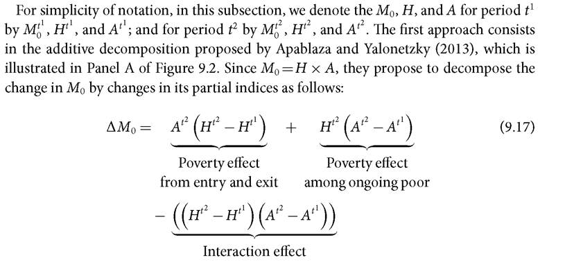
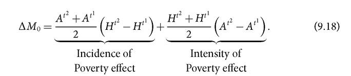
Note that the illustration in Figure 9.2 assumes reductions in M0, H, and A over time, but the graph can be adjusted to incorporate situations where they do not necessarily fall. This approach involves two assumptions. First, the intensity among those who left poverty is assumed to be the same as the average intensity in period t2. Second, the intensity change among the ongoing poor is assumed to equal the simple difference in intensities of the poor across the two periods. The decomposition is completed using an interaction term, as depicted in Panel A of Figure 9.2. This is indeed an additive decomposition of changes in the Adjusted Headcount Ratio (M0). Apablaza and Yalonetzky interpret these changes as reflecting: (1) changes in the incidence of poverty (H), (2) changes in the intensity of poverty (A), and (3) a joint effect that is due to interaction between incidence and intensity (ΔH ? ΔA).
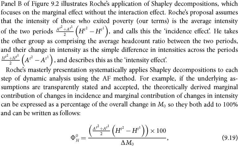
A second theoretical approach corresponds to a Shapley decomposition proposed by Roche (2013). This builds on Apablaza and Yalonetzky (2013) and performs a Shapley value decomposition following Shorrocks (1999).19 It provides the marginal effect of
19 The Shapley value decomposition was initially applied to decomposition of income inequality by Chantreuil and Trannoy (2011, 2013) and Morduch and Sinclair (1998). Shorrocks (1999) showed that it can be applied to any function under certain assumptions.
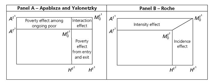
Figure 9.2. Theoretical decompositions
changes in incidence and intensity as follows:
and
φA =
(h'2 + Ht1 (At- — Aμ)) ? 100 ∆M0
(9.20)
To address demographic shifts, Roche follows a similar decomposition of change as that used in FGT unidimensional poverty measures (Ravallion and Huppi 1991) and Shapley decompositions (Duclos and Araar 2006; Shorrocks 1999). This approach, presented in equation (9.21), attributes demographic effects to the average population shares and subgroup M0s across time. Roche argues that if the underlying assumptions are accepted, the overall change in poverty level can be broken down in two components: (1) changes due to intra-sectoral or within-group poverty effect, and (2) changes due to demographic or inter-sectoral effects. So the overall change in the adjusted headcount between two periods, respectively (t2, t1), could be expressed as follows:
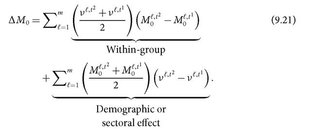
It is common to express the contribution of each factor as a proportion of the overall change, in which case equation (9.21) is divided throughout by ΔM0.
The last columns of Table 9.6 Panel B provide Shapley decompositions for the same five countries. We see that in all cases the Shapley decompositions lie, as anticipated, between the upper and lower bounds. The Shapley decompositions have the broad appeal of presenting point estimates that pinpoint the exact contribution of each partial index to changes in poverty, according to their underlying assumptions, and thus may be used in analyses when empirical accuracy is not required or the assumptions are independently verified. A full illustration of the Shapley decomposition methods using data on multidimensional child poverty in Bangladesh is given in Roche (2013).[238]
9.4
More on the topic Changes over Time by Dynamic Subgroups:
- This chapter provides techniques required to measure and analyse inequality among the poor (section 9.1), to describe changes over time using repeated cross-sectional data (section 9.2), to understand changes across dynamic subgroups (section 9.3), and to measure chronic multidimensional poverty (section 9.4).
- CONTENTS
- Distribution and Dynamics
- ECONOMETRIC SPECIFICATION AND DATA
- Policy Motivation
- SETTING THE SCENE
- THE RESEARCH QUESTION AND METHODS TO EXPLAIN INEQUALITY AND ITS CHANGE
- LMIs AND WAGE INEQUALITY: AN EMPIRICAL ASSESSMENT
- Elements of Measurement Design
- CONTRIBUTIONS TO INTERNET ECONOMICS