Exchange rates and trade performance

The manipulation of exchange rates in attempting to create national competitive advantages is an issue at the forefront of contemporary policy debate. The causes and consequences of exchange rate and currency conflicts are reviewed in some detail.

The chapter concludes by reviewing the operation, over time, of various exchange rate regimes, such as the gold standard, the ‘adjustable-peg’ exchange rate system and freely floating exchange rates.

I The foreign exchange market

The foreign exchange market is the money market on which international currencies are traded. It has no physical existence: it consists of traders, such as the dealing rooms of major banks, who are in continual communication with one another on a worldwide basis. Currencies are bought and sold on behalf of clients, who may be companies, private individuals or banks themselves.

The spot market is used by those who wish to acquire foreign exchange straightaway. Forward markets are used by three groups of people.

1 Those who wish to cover themselves (hedge) against the risk of exchange rate variation. For instance, suppose an importer orders goods to be paid for in three months’ time in dollars. All his calculations will be upset if the price of dollars rises between now and payment date. He can cover himself by buying dollars today for delivery in three months’ time; he thus locks himself into a rate which reduces the risk element in his transaction.

2 Arbitrageurs who attempt to make a profit on the difference between interest rates in one country and another, and who buy or sell currency for­ward to ensure that the profit which they hope to make by moving their capital is not negated by adverse exchange rate movements.

3 Straightforward speculators who use the forward markets to buy or sell in anticipation of exchange rate changes. For instance, if I think that today’s forward rates do not adequately reflect the prob­ability of the dollar increasing in value, I will buy dollars forward, hoping to sell them at a profit when they are delivered to me at some future date.

London is the world’s largest centre for foreign exchange trading, with an average daily turnover of over US $1,100bn.

■ foreign currency options, which give the right (but do not impose an obligation) to buy or sell curren­cies at some future date and price;

■ foreign currency futures, which are standardized contracts to buy or sell on agreed terms on specific future dates; and

■ foreign currency swaps - spot purchases against outright forward currency sales.

Foreign exchange market business in London is done in an increasingly wide variety of currencies: for example, £/$ business now accounts for only 12% of activity. However, trading transactions which do not involve the US dollar are becoming increasingly frequent.

Supply and demand for a currency

Prices of currencies are determined, as on any other market, by supply of and demand for the various cur­rencies. Businessmen wishing to import goods will sell sterling in order to buy currency with which to pay the supplier in another country. Tourists coming to the UK will sell their own currency in order to buy sterling. Other types of transactions, too, will have exchange rate repercussions. For instance, if a German company wishes to buy a factory in the UK it will need to convert euros into sterling, as will for­eign banks who wish to make sterling deposits in London, or residents abroad who wish to buy UK government bonds.

Another way of saying this is that in any given period of time the factors which determine the demand and supply for foreign exchange are those which are represented in the balance of payments account. The demand for foreign exchange arises as a result of imports of goods and services, outflows of UK capital in the form of overseas investment (short and long term), and financial transactions by banks on behalf of their clients.

It is clear from the balance of payments accounts that companies and individuals are not the only cli­ents of foreign exchange market dealers. The Bank of England also buys and sells foreign currency, using the official reserves in the Exchange Equalization Account. In order to reflect on why this might be the case, we have to remember that governments have an interest in the level of the exchange rate, and that they may on occasion wish to intervene in the workings of the foreign exchange market to affect the value of sterling. Indeed, it was estimated that on the day ster­ling was forced to withdraw from the Exchange Rate Mechanism (ERM) (16 September 1992), the Bank of England spent an estimated £7bn, roughly a third of its foreign exchange reserves, in buying sterling. In particular it bought sterling with Deutsche marks (DM) in an unsuccessful attempt to preserve the ster­ling exchange rate within its permitted ERM band.

Historically, the policy stance on this has varied. As we note later in the chapter, it was only after the Second World War that foreign exchange markets began to function freely on a worldwide basis. Govern­ments then had the option of allowing exchange rates to be market-determined, i.e. to ‘float’, or to establish some kind of fixed exchange rate system. The deci­sion was taken at Bretton Woods in 1945 to adopt a fixed exchange rate regime; governments thus com­mitted themselves to continual intervention in the market in order to offset imbalances in the demand and supply for their currencies. The Bretton Woods agreement collapsed in 1972, since when currencies have been allowed to float. However, the European Exchange Rate Mechanism was established in 1979 to restrict the range within which member currencies could float against each other (see Chapter 27), with the ERM eventually leading to the establishment of the euro as the single currency.

We have argued that in everyday terms currency prices are determined by demand and supply on the foreign exchange markets. We must now examine in more detail the forces determining any given exchange rate in the short and long term. As we shall see, all the various theoretical explanations focus on the importance of one or other of the variables contained within the balance of payments accounts. The theor­ies vary only in the time perspective considered. The function of theory is to explain and predict; we shall consider later to what extent recent experience in the UK validates the different theoretical arguments.

Exchange rate definitions

Before we do this, however, we must consider what we mean by ‘the exchange rate’. In a foreign exchange market where exchange rates are allowed to ‘float’, every currency has a price against every other cur­rency. In order to allow for measurability, economists use three separate concepts.

1 The nominal rate of exchange. This is the rate of exchange for any one currency as quoted against any other currency. The nominal exchange rate is therefore a bilateral (two-country) exchange rate.

2 The effective exchange rate (EER). This is a mea­sure which takes into account the fact that sterling varies differently against each of the other curren­cies.

3 The real exchange rate (RER). This concept is designed to measure the rate at which home goods exchange for goods from other countries, rather than the rate at which the currencies themselves are traded. It is thus essentially a measure of competitiveness. When we consider multilateral UK trade, it is defined as:

RER = EER ? P(UK)ZP(F)

In other words, the real exchange rate is equal to the effective exchange rate multiplied by the price ratio of home, P(UK), to foreign, P(F), goods. If UK prices rise, the real exchange rate will rise unless the effective exchange rate falls. We consider below the question of how one might measure this definition empirically.

Nominal exchange rate

Table 25.1 outlines the nominal rate of exchange for sterling against a variety of other currencies (columns 1 to 5) and the overall effective exchange rate (EER) against a ‘basket’ of other currencies (column 6). Of course, from 1 January 1999 onwards the French franc, German mark and Italian lira were replaced by the euro.

We can see from Table 25.1 that the pound ster­ling varied in both directions in terms of its nominal exchange rate against the US dollar over the period 1997-2007, but rose overall with £1 worth $1.64 in 1997 but $2.00 in 2007. However, since 2007 the pound sterling has fallen sharply against the US dollar. The nominal exchange rate for the pound sterling against the euro has fallen consistently over the period 1999-2010, with a particularly sharp fall since 2007. A sharp fall in the nominal exchange rate for the pound sterling against the Japanese yen can also be observed in the period since 2007.

Impacts of a change in the nominal exchange rate A fall in these nominal exchange rates for sterling since 2007 in particular is helping to make UK exports to these countries cheaper (in the foreign cur­rency) and imports dearer (in sterling). For example, in 2007 an American resident would have had to give up $2.00 for each pound, whereas by 2010 he or she would have needed to give up only $1.51 for each pound. British goods and services would therefore have cost less in dollar terms in 2010 than in 2007. We can illustrate the above using data from Table 25.1:

Table 25.1 Sterling exchange rates, 1997-2010.

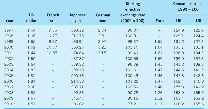
*End of first quarter.

Note: Figures have been rounded to 2 decimal places. The annual sterling effective exchange rate figures were calculated by averaging the daily values sourced from the Bank of England's Interactive Database.

Source: Adapted from Bank of England (2010) Statistics Interactive Database: Interest and exchange rates, April 3rd. Reprinted with permission.

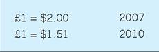
A £100 export from the UK to the US cost $200 in the US in 2007, but costs only $151 in 2010. An import from the US costing $200 would sell for £100 in the UK in 2007 but a higher £132.5 in 2010.

We can therefore conclude that the exchange rate is a key ‘price’ affecting the competitiveness of UK exporters and UK producers of import substitutes.

■ A fall (depreciation) in the sterling exchange rate makes UK exports cheaper abroad (in the foreign currency) and imports into the UK dearer at home (in £ sterling)

■ A rise (appreciation) in the sterling exchange rate makes UK exports dearer abroad (in the foreign currency) and imports into the UK cheaper at home (in £ sterling)

Effective exchange rate (EER)

Of course, UK trade with the US is only a part of UK external transactions. The sterling effective exchange rate (EER) is a weighted average of the various national currencies involved in trade with the UK, the weights given to each national currency depending on the relative importance of UK trade with each of these nations. Currently, the euro has a weight of over 50%, compared to less than 20% for the dollar when calculating the sterling EER, reflecting the relative importance of these areas in UK trade.

As we can see from Table 25.1, the sterling EER has varied in both directions, but overall has fallen by almost 33% since 1998. This suggests a considerable boost to the competitiveness of UK exporters and UK producers of import substitutes over the past 12 years. As we noted in Chapter 1 (p. 19), a fall in the relative exchange rate will, other things equal, reduce a coun­try’s relative unit labour cost (RULC), the single most widely used measure of international competitiveness.

But does the recorded fall in both nominal and effective exchange rates for sterling really mean that UK goods had become more competitive on world markets? Of course the answer depends not only on changes in the exchange rate but on relative inflation rates between the UK and the countries with which we are comparing it. In other words, we must exam­ine the real exchange rate.

Real exchange rates (RER)

Returning again to the bilateral exchange rate between sterling and the US dollar, we can now investigate the real exchange rate (RER) between the two currencies from 1997 to 2010. As we can see from Table 25.1, although the nominal (bilateral) exchange rate between sterling and US dollar fell sub­stantially over the period, consumer price inflation was somewhat higher in the UK than in the US.

Using the information in Table 25.1 on nominal exchange rates and UK/US consumer prices, we can work out the RERs between pound sterling and US dollar for 2007 and 2010:

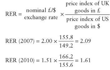
The fall in the RER ($/£) from 2.09 in 2007 to 1.61 in 2010 clearly indicates that by 2010 fewer dollars are needed to be exchanged for each £1 worth of UK products bought in the US. Although inflation was higher in the UK than in the US over the period, the fall in the nominal sterling exchange rate against the US dollar has more than offset the higher UK infla­tion. Whilst sterling depreciated against the dollar by some 25% [(0.49/2.00) ? 100] over the period using nominal exchange rates, it only depreciated by some 23% [(0.48/2.09) ? 100] over the period using real exchange rates. In other words, the loss of competi­tiveness because of higher UK inflation eroded some of the exchange rate gains between UK and US pro­ducers, though these still remained substantial.

I Exchange rate determination

We can distinguish four theoretical approaches to exchange rate determination. It must be emphasized that these are in no sense ‘competing’ theories. They are simply different ways of looking at what deter­mines the exchange rate, depending on whether we are interested in the short run or the long run, in immediate or more fundamental determinants, and on what we consider to be the most empirically rele­vant factors at any given time.

Exchange rates and the balance of trade

The traditional approach sees the exchange rate simply as the price which brings into equilibrium the supply and demand for currency arising from trade in goods and services and from capital transactions, as explained above. This approach was formulated in the 1950s when capital flows were small in relation to trade flows, and hence its major use is to illustrate the interrelationship between current account flows and exchange rate changes. Nevertheless, it can also accommodate capital account transactions. It is essentially a perspective which concentrates on short­run influences.

Figure 25.1 shows that the demand for pounds will increase as the price falls. This is because customers abroad will perceive that the price of UK exports has fallen in their own currency as sterling depre­ciates, increasing their demand for UK exports and therefore for pounds with which to buy them. The supply of pounds will rise as the price of sterling rises because the price of imports in sterling falls as the

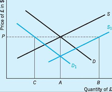
Fig. 25.1 The foreign exchange market.

pound strengthens. With cheaper imports, UK con­sumers now buy more imported items and firms exchange more pounds in order to buy these imports.¹

Demand and supply curves can shift for a number of reasons. A shift (increase) in supply from S to S₁ might be due to a change in tastes in favour of foreign goods. A shift (decrease) in demand from D to D₁ might occur because UK interest rates had fallen, leading to a decrease in the demand for pounds as investors switch their funds out of the UK money markets. In either of these cases, there will be a fall in the exchange rate below its original level, P. In a floating exchange rate system the rate will be allowed to fall. Should the monetary authorities wish to keep the exchange rate at its original level, they will be obliged to buy sterling. If the supply of sterling increases to S₁, they will buy up the excess quantity AB; if the demand for sterling has fallen to D₁, they will make up the shortfall by buying up quantity CA. In either case, the price reverts to its original level.

This view of exchange rate determination predicts that the exchange rate will alter in response to macro­economic policy, because the demand for imports (and hence the supply of pounds) will depend in part on the level of income. Fiscal policy, with its impacts on the equilibrium level of national income, will thus affect the exchange rate. So too will monetary policy as short-term capital flows (and hence both demand and supply of pounds) are seen as being sensitive to interest rate changes. Both fiscal and monetary policy will therefore have exchange rate repercussions. Expansionary policies, whether fiscal or monetary, which raise levels of income and employment will cause the S curve to shift to S₁, as imports rise with income. Such policies may cause a balance of pay­ments deficit and a fall in the exchange rate. The converse will be the case when fiscal or monetary policies are contractionary. Where fiscal and mone­tary policies alter interest rates in a downward direc­tion (as, for instance, if public borrowing is reduced so that fewer bonds need to be issued, bond prices rise and yields fall, or interest rates are reduced directly by the monetary authorities), capital outflows will be triggered - S will move to S₁ as people move their money out of UK financial markets; at the same time D will fall to D₁ as investment in UK money markets is no longer forthcoming.

What this model does not enable us to do is to pre­dict the overall effect of any given policy stance. In the case of an expansionary monetary policy, spending

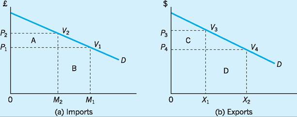
Fig. 25.2 Marshall-Lerner elasticity conditions.

will increase and interest rates will fall, the supply of pounds will increase in both cases and the exchange rate will fall. But in the case of an expansionary fiscal policy, expansion may be associated with an increase in government borrowing, which will lead to a fall in bond prices (as the supply of bonds increases) and a rise in the interest rate. The effect on the exchange rate will then be ambiguous, depending on the mar­ginal propensity to import from a rise in income in relation to the interest elasticity of capital flows.

Marshall-Lerner elasticity condition

We have seen how the traditional explanation of exchange rate determination is based on balance of payments flows. However, there is also a ‘feedback’ effect in that these flows, in particular flows of imports and exports, are themselves partly deter­mined by the level of the exchange rate. Suppose that an exogenous disturbance, such as a change in gov­ernment policy, leads to a balance of payments deficit and a consequent fall in the exchange rate. Since the demand for exports and imports is dependent on their price, will the new exchange rate level result in a further deterioration in the balance of payments and a further fall in the exchange rate, or will the balance of payments improve and the exchange rate return to its former level?

The answer to this question depends on the elas­ticities of demand for imports and exports. The ‘elas­ticities’ approach to balance of payments adjustment predicts that if the sum of the elasticities of demand for imports and exports is greater than one (the Marshall-Lerner condition) then the balance between the change in export earnings and import expenditure will be such as to improve the balance of payments, and the exchange rate will rise in consequence.

The Marshall-Lerner condition can be outlined further by reference to Fig. 25.2 where, following a depreciation of the pound, the price of imports increases and the price of exports decreases. In Fig. 25.2(a) a depreciation of the pound has resulted in a rise in the sterling price of imports from P₁ to P₂ and reduced their demand from M₁ to M₂. This leads to an increase in sterling expenditure on imports of area A but a reduction in sterling expenditure on imports of area B. There will be an overall reduction in expen­diture on imports of (B - A) if the demand for imports is elastic. In Fig. 25.2(b) the depreciation of the pound has resulted in a reduction in the foreign ($) price of exports from P₃ to P₄ and an expansion in the demand for exports from X₁ to X₂. This will lead to a reduction in expenditure by foreigners on UK exports by area C, but at the same time there will be a rise in expenditure by foreigners on UK exports of area D. There will be an overall increase in expen­diture by foreigners on UK exports of (D - C) if the demand for exports is elastic.

In terms of the balance of payments, the effect will have been an improvement of (B - A) + (D - C), which will be greater the higher the respective elas­ticities of demand for imports and exports. However, it can be shown that the cut-off value for these re­spective elasticities is where the sum of their values equals 1. In this situation a fall (depreciation) in the exchange rate will leave the balance of payments unchanged. However, if the sum of these respective

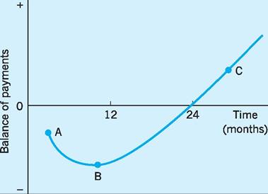
Fig. 25.3 ‘ J' curve effect.

elasticities is less than 1, then a fall (depreciation) in the exchange rate will cause the balance of payments to deteriorate. Only if the sum of these elasticities is greater than 1 and the Marshall-Lerner condition is fulfilled, will a depreciation (eventually) improve the balance of payments.

In practice the following factors may influence the balance of payments outcome from any given fall in the exchange rate:

■ Trade adjustments take time. The exchange rate may adjust instantaneously, but traders take time to adjust their orders. The initial effect of a depre­ciation may therefore be to make the deficit larger as export demand is slow to increase at new lower prices, and importers fail to cut back their pur­chases. There will thus be a ‘J-curve’ effect (see Fig. 25.3) as the balance of payments deteriorates (A to B) before it improves. It has been estimated from previous falls in the exchange rate that it is only during the second year after the devaluation/ depreciation that the gain in export volume offsets the loss in revenue due to lower export prices.

■ In a floating exchange rate regime exchange rates will alter again in the time it takes for these adjustments to be made. Stability is therefore unlikely to occur.

■ The analysis takes no account of supply condi­tions. In a full employment situation it may not be possible to cope with the increased demand both for exports and for import-competing goods, so that the beneficial effect of a depreciation may not be realized because of supply constraints.

■ The fall in the exchange rate will increase home prices, because import prices have risen, and may therefore cause an inflation which will offset to some extent the positive balance of payments effects of the depreciation of the exchange rate.

■ It is assumed that only prices determine trade flows. In fact, there are several reasons why trade flows may be unresponsive to exchange rate changes. Quality and product differentiation are often more important in determining trade flows than prices.

■ The analysis takes no account of the effect of exchange rate changes on capital flows. If these latter are quantitatively unimportant this does not matter, but since they currently play a very large part in exchange rate determination the usefulness of the elasticities approach is weakened.

The ‘traditional’ analysis of exchange rate deter­mination, which sees exchange rates as a function of the current balance of payments position, became less useful as historical circumstances have changed. Two major developments after the 1950s made it neces­sary to consider alternative theoretical approaches.

One of these was the growing importance of cap­ital flows in the balance of payments accounts. These flows of international investment were partly caused by capital formation by multinational companies (see Chapter 7) but were also due to increasing prefer­ences by asset holders for holding foreign assets as capital restrictions were eased. The last of these restrictions vanished in 1979 when the UK abolished exchange control. The other, later, development was the advent of worldwide inflation in the 1970s. The traditional view outlined earlier took no account of internal price changes when analysing exchange rate variations. In fact, in an inflationary situation internal and external price changes are interactive.

These two developments led to the monetary and portfolio approaches to exchange rate determination on the one hand, and to the revival of the purchasing power parity (PPP) theory on the other. Because the monetary and portfolio approach hinges on the valid­ity of the PPP theory, we deal first with purchasing power parity.

Purchasing power parity

This theory originated in the nineteenth century, and was used in the 1920s to discuss the correct value of currencies in relation to gold. In general terms, the proposition states that equilibrium exchange rates will be such as to enable people to buy the same amount of goods in any country for a given amount of money. For this to be the case, exchange rates must be at the correct level in relation to prices in the dif­ferent countries. In order to state the proposition more rigorously, we must assume that goods are homogeneous (or that there is only one good), also that there are no barriers to trade or transactions costs, and that there is internal price flexibility. The ‘law of one price’ will then ensure that the price of a good will be equalized in domestic and foreign cur­rency terms. For instance, the price of a car in the UK in sterling must be equal to the price of a car in US dollars times the exchange rate (the sterling price of dollars). If the exchange rate is too high or too low, it will adjust if exchange rates are flexible. If they are fixed, internal prices will adjust as there is an excess of demand in one country and a shortfall in the other. There are two versions of the proposition.

1 The ‘absolute’ version of PPP predicts that the ex­change rate (E) will equalize the purchasing power of a given income in any two countries, so that

E = P(UK)∕P(US)

2 The ‘relative’ version of the principle states that changes in exchange rates reflect differences in relative inflation rates. If internal prices rise in one country relative to another, exchange rates will adjust (downwards) to compensate.

It is easy to see how the existence of high inflation rates in the 1970s increased the attractiveness of this theory as an explanation of exchange rate determina­tion, because the theory concentrates on showing the relationship between exchange rates and relative price movements, unlike the more traditional view which, as we have seen, had nothing to say about prices. However, what can we say about the empir­ical usefulness of the principle? Let us consider the problems of applying the principle first, and then look at the extent to which it was in fact successful in explaining exchange rate changes.

A number of damaging criticisms of the theory can be made.

■ The major problem relates to the choice of price index used to give empirical content to the theory. Any overall price index includes non-traded as well as traded goods, and inflation rates may be differently reflected in these sectors, hence render­ing the index unusable. Even the use of export price indices is problematic because the profitabil­ity element in export prices may vary over time. The appropriate measure would appear to be a measure of unit labour costs normalized as between countries (relative normalized unit labour costs - RNULC) which reflects differences in wage costs per unit of output and thus includes productivity measures.² The RNULC measures are the most accurate way of assessing the relative competitive strength of different countries in the traded goods sector (see also Chapter 1).

■ It is difficult to discuss an ‘equilibrium’ exchange rate without reference to some base year. The choice of representative year can pose problems in a world where inflation rates vary constantly.

■ Factors other than the prices of traded goods can affect the exchange rate. Barriers to trade such as tariffs can exist. Tastes can change, incomes can change, technology can change. The classic example of the latter is the effect on the exchange rate of North Sea oil.

■ Although in the long run the PPP theory may have some validity, exchange rates in the short run are more likely to be dominated by the effects of capital flows, particularly short-run flows. In other words, exchange rates may ‘overshoot’.

Quite apart from these particular criticisms, it is doubtful whether the PPP theory provides us with an adequate explanation of changes in the sterling exchange rate. The theory would predict that if prices rise faster in the UK than in other countries the resul­tant trade deficit should cause a fall in the exchange rate. We can test this by examining the relationship between the EER and RNULC. When costs rise the UK is becoming less competitive, so we might expect to see a consequent fall in the EER if the ‘relative’ version of the PPP theory holds. In other words, there should be an inverse relationship between the two measures. However, empirical evidence is rather weak in this respect, with relative prices (proxied by unit labour costs) and the EER often tending to move together rather than inversely. There are various possible explanations for this.

■ Price elasticities for imports and exports may not be such as to cause the exchange rate to improve

with a rise in competitiveness. In fact, with a float­ing exchange rate a rise in competitiveness may cause the exchange rate to fall (the J-curve effect).

■ The EER is influenced by trade in invisibles and by capital flows as well as by the relative prices of manufactured goods entering into trade.

■ Price competitiveness is not the only factor affect­ing trade flows. Non-price competitiveness is also an important determinant. In other words, the crucial assumption of the ‘law of one price’ - that of homogeneous goods and services - does not hold in the real world.

We must also realize that RNULCs are themselves influenced by the EER. This is because costs of pro­duction in the UK will rise faster than those in other countries if the EER depreciates. Raw materials will become more expensive, production costs will rise, and any resulting (cost-push) inflation may trigger wage demands to respond to the price rises, and RNULC will rise in consequence.

We may sum up by saying that the usefulness of the PPP theory as a theory of exchange rate deter­mination is probably best thought of in a long-run context when changes in relative prices between countries represent the workings of inflationary forces rather than transient ‘real’ effects such as changes in tastes or technology. However, even in the long run it is still not possible to say whether relative price shifts determine exchange rate movements, or whether exchange rate changes influence price movements.

North Sea oil and the exchange rate

We have argued that little of the variation in the EER can be explained by UK price competitiveness. Other factors have been more important: one of these has been the fundamental change in technological possibilities resulting in the ability to undertake deep water oil exploration and extraction, providing the context for the advent of North Sea oil. North Sea oil came on stream in 1976, and the UK became self-sufficient in oil by 1980. This has been perhaps the main reason why over various periods of time since then, the EER has risen in spite of a loss of competitiveness.

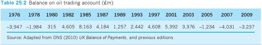
There are three ways in which oil production has improved the balance of payments.

First, since 1976 the UK has been an exporter of oil and has reduced its own dependence on imported oil. As we can see from Table 25.2, the oil trading balance improved steadily from 1976 onwards, and moved into surplus in 1980. However, after 1985 oil production began to decline in volume, and this was reflected in the reduced oil surplus from 1985 to 1993. Nevertheless, a recovery in world oil prices, new oil fields yielding extra output and the lower price of oil exports (after sterling depreciated on leaving the European ERM in 1992) all contributed to an improvement in the oil trade balance in the mid-1990s and early years of the new millennium. There has been a tendency for oil prices to rise in recent years, due partly to uncertainties as to future supplies of oil (e.g. Gulf War 2, hurricanes and oil spills in the Gulf of Mexico) and partly to more effective restrictions on the supply of oil from the OPEC oil cartel.

Second, the inflows of capital needed to fund investment in the oil industry helped the UK balance of payments in the 1970s. However, this positive effect has to some extent been offset since then by outflows of interest, profits and dividends as com­panies remit their gains back to the country of origin.

Third, the popularity of sterling rose as inter­national asset holders speculated on the strength of sterling deriving from the (then) favourable oil trad­ing balance. Such problems have raised the profile of sterling as a ‘petro-currency’, attractive to investors at a time of higher oil prices.

The net effect of the balance of payments impact of North Sea oil is likely to have been sufficiently favourable to keep the exchange rate higher than it would otherwise have been over the past few decades.

The monetary approach to exchange rate determination

As we saw earlier, the growth in importance of cap­ital account transactions led to attempts to explain the determination of the exchange rate by analysing financial flows between countries. The monetary approach to exchange rate determination, developed in the early 1970s, sees the exchange rate as the price of foreign money in terms of domestic money, deter­mined in turn by the demand for and supply of money. If people are not willing to hold the existing stock of money there will be a shortfall in demand for it and its price will fall in relation to the currencies of other countries. What it in fact argues is that balance of payments, and hence exchange rate move­ments, are simply reflections of disequilibria in money markets.

Money is thought of as being an asset, the demand for which depends on income and interest rates. If the central bank in a country increases the money supply, income and interest rates remaining unchanged, people will be unwilling to hold more money and so the excess money holdings will be used to buy more goods from abroad. The result will be a balance of payments deficit and downward pressure on the exchange rate. If the authorities intervene to support the currency they will lose reserves, and so the increase in the money supply will be exactly offset by a reduction in the external component of the money stock (see Chapter 20). On the other hand, if exchange rates are flexible, the fall in the exchange rate will simply result in internal inflation (as the price of imports rises) which will exactly cancel out the original increase in the money supply.

Suppose now that there is no increase in the money supply, but that exogenous factors cause a change in the demand for money. Suppose incomes rise: the increase in demand for money balances will then lead to an appreciation of the exchange rate as less money is available for imports. Or suppose inter­est rates rise: the demand for money balances will be reduced, people will spend the money on imports, the exchange rate will fall and home inflation will result. (Note that the prediction here is at variance with the usual assumption that a rise in interest rates will cause an appreciation of the exchange rate because capital flows will be attracted into the country.)

The monetary approach to exchange rate determin­ation, incorporating as it does a whole new perspective on the role of money in the balance of payments, provides a monetarist explanation of exchange rate determination. Its strength lies in the fact that it recognizes the importance of asset market changes in determining the exchange rate, as opposed to concen­trating merely on the importance of current account flows in the short or long term, as the previous approaches did. That perspective allows for the possibility of introducing the question of the effect of expectations, which is essential if we are to explain exchange rate volatility. However, in evaluating the usefulness of this approach we must first of all remember that the validity of the argument rests on very limited assumptions:

■ The demand for money is a stable function of real income and interest rates.

■ Prices are determined by the world price level and the exchange rate, i.e. the PPP theory holds.

■ There is full employment domestically.

The validity of these assumptions may be criticized on several grounds:

■ The impact of a monetary disturbance on prices and hence the exchange rate may not be predict­able in the short run because of the instability of the velocity of circulation (see Chapter 20).

■ Exchange rates do not conform to the naive PPP model.

■ Changes in the money stock may produce short­run changes in output (see Chapter 20) which may make it difficult to identify ultimate effects on prices and the exchange rate.

It may help to remember the restrictiveness of these assumptions when we examine some of the implications of this monetarist view. For instance, it is clear that the theory implies that there is no need to have a balance of payments policy, since deficits are self-correcting, because increases in the money stock are reversed either by exchange market intervention or by the effects of resultant price rises. But perhaps the major problem with the monetary approach to exchange rate determination, and certainly the cen­tral problem when it comes to any empirical testing of its usefulness as an explanatory device, is that it considers there to be only one asset - money - which affects exchange rate determination. This is clearly not the case in practice. We must therefore look to a wider interpretation of asset-holding behaviour if we are to account for the actual behaviour of the exchange rate.

The portfolio balance approach to exchange rate determination

The portfolio balance approach to exchange rate deter­mination sees exchange rates as determined mainly by movements on the capital account of the balance of payments. However, it recognizes that there are a wide variety of assets represented by these transactions. Wealth holders will hold their assets in domestic and foreign securities as well as money, and their asset preferences will be determined by their assessment of the relationship between risk and return on these assets. Given the difference between domestic and foreign rates of return, the exchange rate will be determined by investors’ assessment of the degree of substitutability between domestic and foreign assets. If domestic interest rates rise, the extent to which this will cause an inflow of capital and a consequent appreciation of the exchange rate will depend on investor expectations. If expectations change, so that the perceived relationship between risk and return alters, the exchange rate will vary accordingly.

This approach, which was developed in the mid- 1970s, represents the ‘state of the art’ in exchange rate theory. It does not discount the influence of the current account in trend movements of the exchange rate, but it does suggest a plausible explanation for the observed short-run variability in the exchange rate. Exchange rates may vary sharply in response to asset-switching behaviour in the face of changing rates of return and expectations. Adherents of this view would argue that the major exchange rate changes of September 1992 were largely caused by asset-switching behaviour by portfolio holders. For example, once expectations moved sharply against the lira and pound sterling holding their central par­ities in the ERM, it became a ‘low-risk’ one-way bet to move out of those currencies into ‘harder’ curren­cies such as Deutsche mark and yen.

Short-term capital flows and the exchange rate

Here we consider the way in which the exchange rate is influenced by short-term capital flows. These consist mainly of borrowings from, and lending to, overseas residents by banks. Such short-term capital flows respond primarily to interest rate differentials. Asset switching between countries will take place so long as the interest rate differential is greater than any expected changes in the exchange rate. What happens is that if interest rates rise in, for instance, the US, people will buy dollars in order to invest in US money markets. This will drive the dollar rate up, but as people realize their gains by selling dollars the dollar rate will come down again. It is possible to try and hedge against potential loss by selling dollars bought today on today’s forward market for delivery at some future date, but that will in turn drive today’s for­ward rate down. In a perfect market the rise in dollar spot rate and the fall in forward rates (as investors try to make sure of their future gains today) will be just sufficient to cancel out the advantages of rising inter­est rates. But markets are never perfect, and some arbitrage is always possible.

We have no firm empirical evidence for such behaviour on the part of asset-holders. There should be a positive correlation between interest rate differ­entials and exchange rates, as people switch funds into the UK when interest rates rise relative to US interest rates, thereby driving up the sterling exchange rate. However, empirical evidence as regards the UK/ US interest rate differential shows as much evidence of negative as of positive correlation. There are vari­ous reasons for this. One is that the positive effect of interest rate differentials on the exchange rate may be outweighed by exchange rate expectations. For instance, in the period 1980-82, when interest rate differentials were very low because both the UK and the US had high interest rates, the UK exchange rate was high because people believed that a petro­currency such as sterling would remain strong.

Expectations about future exchange rates are formed by assessments about the potential demand for and supply of sterling. If asset-holders see that the UK has a combined current and capital account deficit, they will expect the exchange rate to fall, and will move their money out of sterling, thereby exerting a further downward pressure on sterling. If the authorities do not wish this to happen, they must raise interest rates so that they are higher than those of other countries by a margin sufficient to attract funds into sterling.

Of course, it is never possible to predict the effect on capital flows, and hence on the exchange rate, of any given interest rate differential. Capital flows will be more or less responsive, depending on the strength and the nature of expectations. Lacking adequate information in an imperfect market, speculators tend to be influenced by any item of information, however irrelevant. Money supply figures, political develop­ments at home and abroad, unsuccessful summit meetings - all these tend to trigger behavioural responses in terms of flows of ‘hot’ money in and out of sterling. Exogenous shocks, such as the con­sequences of oil price rises, or the threat of inter­national conflict, may also lead to major flows of short-term capital. It may happen that, in spite of high interest rates, the exchange rate does depreciate. In this case, there will be consequent structural changes both in competitiveness and in real rates of return on long-term investment.

Expectations would certainly seem to have out­weighed interest rate differentials in September 1992, when a number of ERM currencies came under intense speculative attack. Despite sharp rises in Italian and UK interest rates, for example, the spe­culative pressure against the lira and pound was sustained. In the case of the UK, interest rates rose an unprecedented five percentage points (from 10% to 15%) within 24 hours. Even this, together with an estimated expenditure of £7bn by the Bank of England (roughly one-third of total UK reserves) in purchasing sterling, and further support of over £2bn by the Bundesbank, could not withstand the continued speculative pressure. Eventually the UK was forced to withdraw from the system altogether (see Chapter 27) and the Italians had to reduce the central parity of the lira within the system. payments is an accounting identity, so that there is a corresponding minus sign (deficit) for every plus sign (surplus), with the net total always zero, except for errors and omissions. In other words, the balance of payments corresponds to a zero sum game, and every ‘win’ for one party involves, by definition, a ‘loss’ for another party.

The current account balance in Fig. 25.4(a) repre­sents the absolute value (in $bn) of the deficit (-) or surplus (+) for trade in goods and services fore­cast for 2010 by the IMF in October of that year. Figure 25.4(b) presents the same data, but as a per­centage of the GDP of the respective countries. Whilst capital inflows (+) and outflows (-) are not shown in the current account balance, the picture is clearly one of major deficit for some countries and major surplus for other countries. Moreover, the 2010 ‘snapshot’ of trade performance reflects a longer term reality for many countries as regards their trade in goods and services, as is suggested by the substantial growth in foreign exchange reserves for a number of countries over the 2000-2010 period shown in Fig. 25.4(c).

While the US has much the largest absolute current account deficit at almost $450bn in 2010, as a pro­portion of GDP that current account deficit is, at around -3%, smaller in percentage terms than for the current account deficits in Spain (-5.1%), Turkey (-5%) and South Africa (-4.2%). Nevertheless, these current account imbalances, where they are persistent as in the case of the US, are believed by many analysts to be unsustainable, even when mitigated to some ex­tent and for some countries by surpluses on the capital account (capital inflows exceeding capital outflows).

I Currency ‘warfare’

There has been much discussion amongst nations, analysts and global institutions as to the ‘dangers’ of currency manipulation for international trade and economic growth. In September 2010 the US House of Representatives passed a law allowing firms to seek tariff protection against countries with under­valued currencies, a key focus of such a law obviously being China.

Figure 25.4 provides useful data for the G20 group of countries which underpins many of these con­cerns. The key point is, of course, that the balance of

Self-correcting mechanisms

As we note below (p. 544) the so-called floating exchange rate regime can, potentially, help avoid the persistent balance of payments deficits and surpluses that are all too prevalent in the global economy. It may be useful at this point to outline the mech­anisms that might be expected to provide a degree of ‘self-correction’ to balance of payments disequilibria, before exploring why such mechanisms seem not to have worked in practice, at least as regards certain major ‘players’ such as the US and China!

The exchange rate should, under a floating exchange rate regime, be responsive to changing balance of payments outcomes, depreciating for deficit countries

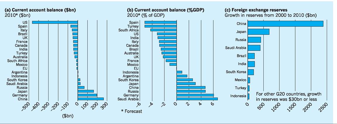
Fig. 25.4 Balance of payments, foreign exchange reserves and currency implications.

Source: Balance of payments, foreign exchange reserves and currency implications, Financial Times, 03/11/2010 (Wolf, M.).

538 CHAPTER 25 EXCHANGE RATES AND TRADE PERFORMANCE

and appreciating for surplus countries. Yet despite its huge ($200bn) bilateral balance of payments surplus with the US in 2009/10, the Chinese yuan barely appreciated against the US dollar over that period, rising by less than 1% throughout the whole period! The People’s Bank of China (PBOC), the country’s central bank, administers China’s exchange rate policy, and has clearly acted to stabilize the yuan at close to its current rate, rather than permitting the sharp appreciation of the yuan which might other­wise occur in a free-market system.

Currency-related conflicts

At least three areas of concern were identified in the G20 meeting in October 2010 in South Korea.

First, the allegedly undervalued yuan, with many countries (especially the US) arguing for a significant appreciation, making Chinese exports dearer abroad and imports cheaper within China.

Second, quantitative easing (see Chapter 20, p. 419) and other aspects of monetary policy in the advanced industrialised economies has increased the supply of sterling, dollar, yen and other currencies on foreign exchange markets, tending to lower these countries’ exchange rates. With the increase in liquidity, rise in prices and lower interest rates often associated with quantitative easing, China and others argue that these policies artificially depreciate other country exchange rates (a relative appreciation for the yuan). Also the low interest rates and fear of investors that the exchange rates of countries engaged in quantitative easing will fall, both combine to lead to major capital outflows from these advanced economies to the emerging economies such as China and India, putting upward pressures on their exchange rates.

Third, in order to prevent exchange rate apprecia­tion, emerging and other capital receiving economies are intervening more actively, selling their own cur­rencies and buying foreign currencies and/or impos­ing taxes on foreign capital inflows. Brazil doubled its tax on foreign purchases of domestic debt in 2010 and Thailand announced a new 15% withholding tax for foreign investors in its bonds in October 2010.

What is seen by most analysts of the IMF, G20, OECD, World Bank and others is an urgent need to rebalance global demand for products by switching spending away from the indebted advanced econom­ies and towards the emerging economies.

‘Appropriate’ exchange rates

Interestingly, the communique from the October 23 meeting of G20 finance minutes in South Korea, included the following statement:

Persistently large (balance of payments) imbalances, assessed against indicative guidelines to be agreed, would warrant an assessment of their nature and the root causes of impediments to adjustment as part of the Mutual Assessment Process, recognizing the need to take into account national or regional circumstances, including [those of] large commodity producers (G20 communique, 2010, October).

Despite its complexity, it is interesting to note that both China and the US could agree the above statement. Of course much depends on the discussions regarding implementing this approach, especially agreeing the ‘indicative guidelines’! The US has suggested that 4% of GDP might be the target for determining which are the countries with ‘persistently large imbalances’ and that both surplus and deficit countries breaching this threshold would have an obligation to adjust.

‘Big Mac’ index

The homogeneous and globally consumed ‘Big Mac’ has been used for some time as a useful indicator of the extent to which a currency is under- or overvalued. The index is based on the idea of PPP, i.e. that a currency’s price should reflect the amount of goods and services which can be bought with that currency. Since it only costs a Chinese consumer 14.5 yuan to buy a Big Mac and a US consumer $3.71, then 1 yuan should exchange against $0.26 on the foreign ex­change market. In fact 1 yuan exchanged against $0.15 on the 13th October date of the Big Mac index, suggesting that the yuan is undervalued by around 42% [(0.11/0.26) ? 100].

Figure 25.5 uses this approach to identify which currencies are under and overvalued. As we can see, using the US as comparator, Switzerland, Brazil, the Euro area, Canada and Japan are overvalued against the US dollar, and China, Malaysia, Russia, Thailand, Mexico, South Africa, South Korea, Singapore and the UK are undervalued.

IMF approach

The IMF has proposed a rather complex method for its own assessment of under- and overvaluation of an

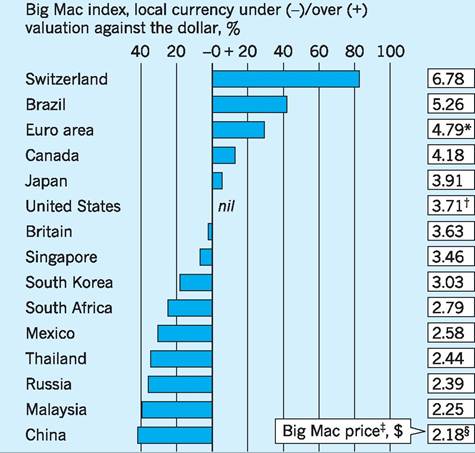
Fig. 25.5 ‘Big Mac' Index.

*Weighted average of member countries; ^tAverage of four cities; ^tAt market exchange rate (Oct 13th); ^sAverage of two cities. Source: The Economist (2010), October 14.

exchange rate. This method incorporates different, but related, approaches with a key element being a calculation of the RER that would be necessary to bring the current account balance into line with a ‘norm’ identified by the IMF for that country. This ‘norm’ is based on the country’s growth rate, its income per capita, demographic characteristics and budget balance. Another element in the calculation involves establishing the RER which would stabilize the country’s foreign assets and liabilities at a ‘rea­sonable’ level. This attempt to find a universally accepted definition of under- or overvaluation of a currency is very much in its infancy.

Economic policy and the exchange rate

It has become increasingly clear that there is a direct relationship between changes in the exchange rate and the rate of inflation, because the price of imports enters into the Consumer and Retail Price Indices (CPI and RPI) in different ways. We can illustrate this as follows. In Fig. 25.6 we consider in some detail the impact of a sterling depreciation on UK import prices. Sterling depreciation will raise the cost, expressed in sterling, of imported items. However, both the magnitude and the speed of price rise will vary with the type of import. This can be illustrated for the 1980s by reference to a Bank of England short-term forecasting model. As we can see from Fig. 25.6, the full effect of the sterling depreciation on import prices will only be felt after more than two years. Imported fuel and industrial material prices will, with less elastic demands, respond most substan­tially and most rapidly to the depreciation. This is in part because the less elastic is demand, the easier it is to pass on cost increases to consumers. Imported finished goods prices rise by a smaller amount, and less quickly, because some of these goods face exten­sive competition on home markets, i.e. face more elastic demand curves. Imported food prices will tend

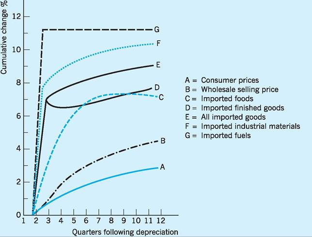
Fig. 25.6 I mpact on prices of a 10% depreciation.

Notes:

1 A 10% depreciation of sterling against the dollar is equivalent to an increase of 11.1% in units of sterling per dollar. As it is the latter rate which is relevant in this context, the 10% depreciation leads eventually to a rise slightly greater than 11% in some import prices.

2 The bank's short-term model assumes no wages response. The exchange rate is assumed to remain 10% below the level it would otherwise have been.

to be less affected, at least initially, because of the operation of the Common Agricultural Policy.

The final effect on consumer prices can be seen to be about one-quarter of the sterling depreciation, and then only after more than two years. For any depreciation, the final effect on consumer prices will depend on a number of factors:

■ the import content of production;

■ the extent to which cost increases can be passed on

to consumers, i.e. price elasticity of demand;

■ the import content of consumption; and

■ the sensitivity of wage demands to cost-of-living increases.

Figure 25.6 is drawn on the assumption of no wage response, i.e. that the sensitivity of wage demands to cost-of-living increases is zero. Any such response would increase wholesale and consumer prices still further.

Whereas a fall in the sterling exchange rate will increase inflation, a rise in the exchange rate will reduce it. There is, of course, another side to the picture. A high sterling exchange rate, although help­ing the fight against inflation, may adversely affect output and employment. United Kingdom producers may now find it more difficult to sell their goods and services, first, because competition from cheaper imports drives them out of home markets and, sec­ond, because UK exports become expensive on foreign markets. Much of the deindustrialization of the early 1980s was attributed to the high pound, and again in the period 1996-2007 (see Chapter 1).

The adherence of governments to a policy of high exchange rates has often been based on a belief that high exchange rates help fight inflation by mak­ing imports cheaper, and that on the export side reliance could be placed on the ‘law of one price’. In other words, British manufacturers, seeing that they could not sell on world markets unless they observed world prices for their products, would restrain the rate of growth of labour costs, thereby raising exports and further contributing to the fight against inflation.

It will be useful to conclude this chapter by review­ing the various types of exchange rate regime which have operated over time, before considering the system under which the UK currently operates.

I The gold standard system

As the nineteenth century progressed, and as world trade expanded, the use of gold as a means of inter­national payment broadened to take in almost all the major trading countries. Although a few, such as the US, persisted for some time with silver, by about 1873 (with the passing of the Gold Standard Act in the US) a gold standard payments system could be said to be in effect. The ‘price’ of each major currency was fixed in terms of a specific weight of gold, which meant that the price of each currency was fixed in terms of every other currency, at a rate that could not be altered. The gold standard was therefore a system of fixed exchange rates. Any difficulties for the bal­ance of payments had to be resolved by expanding or contracting the domestic economy. A rather stylized account of the adjustment mechanism will highlight the main features of the gold standard system.

Suppose a country moved into balance of pay­ments surplus. Payment would be received in gold which, because domestic money supply was directly related to the gold stock, would raise money supply. This would expand the economy, raising domestic incomes, spending and prices. Higher incomes and prices would encourage imports and discourage exports, thereby helping to eliminate the initial pay­ments surplus. In addition, the extra money supply would lead to a fall in its price (the rate of interest), encouraging capital outflows to other countries which had higher rates of interest - a minus sign in the accounts. A payments surplus would, in these ways, tend to be eliminated. For countries with payments deficits, gold outflow would reduce the gold stock and with it the domestic money supply. This would cause the domestic economy to contract, reducing incomes, spending and prices. Lower incomes and prices would discourage imports and encourage exports. The reduction in money supply would also raise the price of money (interest rate), encouraging capital inflows - a plus sign in the accounts. Payment deficits would, therefore, also tend to be eliminated. This whole system came to be regarded as extremely sophisticated and self-regulating. Individual countries need only ensure (a) that gold could flow freely between countries, (b) that gold backed the domestic money supply, and (c) that the market was free to set interest rates. Of course, this meant that countries with payment surpluses would experience expanding domestic economies, and those with deficits contract­ing economies.

There seemed to be a general acceptance amongst the major trading nations that currency and payments stability took precedence over domestic production and employment. What was perhaps not realized was that the apparent ‘success’ of the system in the 40 years between 1873 and 1913 was largely due to the additional liquidity provided by sterling balances. The growing value of UK imports had led to an in­crease in the holding of sterling by overseas residents, who then used sterling to settle international debts.

If the supply of gold and other precious com­modities could not keep pace with the expansion of world trade, the obvious alternative was to make use of ‘paper’. In practice, of course, exporters would accept only paper and a ‘paper’ system could be used on a worldwide basis only when it fulfilled a number of useful criteria:

1 It had to be freely exchangeable on a global basis.

2 It had to be available in sufficient quantities.

3 It needed to be of a fixed value which did not depreciate rapidly.

4 Its value, ideally, needed to be guaranteed in terms of some other precious commodity such as gold.

The paper currency, in other words, had to be ‘as good as gold’.

For a brief period in the late Victorian and early Edwardian eras sterling fulfilled the bulk of this role. Sterling continued to play a part in the funding of international debt in what was called the ‘Sterling Area’ well into the 1960s.

Although several attempts were made to revive the gold standard after the First World War, these largely failed. The dominance of the UK in world trade began to fade during this period, restricting the supply of sterling as a world currency. The Great Depression of the late 1920s and early 1930s also encouraged many countries to adopt protectionist measures. In such an atmosphere countries became less willing to abide by the ‘rules’ of the gold standard. Gold flows were restricted, and money supply and interest rates were adjusted independently of gold flow to help domestic employment rather than inter­national payments. Wages and prices became much more rigid as labour and product markets became less ‘perfect’, which further impeded the adjustment mechanism. For instance, any deflation that did still occur in deficit countries led less often to the reduc­tions in factor and product price needed to restore price competitiveness. Countries began therefore to resort more and more to changes in the exchange rate to regain lost competitiveness.

This breakdown of the gold standard system dur­ing the inter-war period found no ready replacement. The result was a rather chaotic period of unstable exchange rates, inadequate world liquidity and pro­tectionism. It was to seek a more ordered system of world trade and payments that the Allies met in Bretton Woods, in the US, even before the Second World War had ended. What emerged from that meeting was an entirely new system, under the aus­pices of the IMF.

I The IMF system

The adjustable-peg exchange rate system

Imbalances in world trading patterns, and imperfec­tions in world money markets have at least three implications:

1 That deficits and surpluses rarely self-correct, so that foreign exchange reserves are required to fund persistent payments deficits.

2 That although surpluses and deficits are supposed to balance as an accounting identity for the world as a whole, in practice surpluses are rarely recycled to debtor countries.

3 That even though in theory the world must be in overall balance, in practice there is a substantial imbalance. As far as these missing balances are concerned, the IMF reported in 1991 a global sur­plus of over $100bn. A number of factors may be involved: time-lags in reporting transactions, the non-recording of arrangements conducted through tax havens, and the problem of using an appropri­ate ‘price’ to evaluate trade deals when exchange rates fluctuate several times between initiation and completion.

In order to settle deficits, theory tells us that deficit countries should be able to run down their foreign exchange reserves, or to borrow from surplus coun­tries. Both methods have, in reality, proved next to impossible. The countries most likely to suffer deficits are those with low per capita incomes and few for­eign exchange reserves. They are also in consequence those with low credit ratings on the international banking circuit, making borrowing from surplus countries difficult. It was in order to solve just these sorts of liquidity problems for deficit countries that the IMF was established. As well as providing foreign currencies in times of need, its other major objective was to promote stability in exchange rates, following the uncertainties of the inter-war period.

Exchange rate stability

Under the IMF system, each country could, on join­ing, assign to itself an exchange rate. It did this by indicating the number of units of its currency it would trade for an ounce of gold, valued at $35. The dollar was therefore the common unit of all exchange rates. A country had a ‘right’ to change its initial exchange rate (par value) by up to 10%. For changes in par value which, when cumulated, came to more than 10%, the permission of the IMF was required. The IMF would give such permission only if the member could demonstrate that its payments were in ‘fundamental disequilibrium’. Since this term was never clearly defined in the Articles of the IMF, any substantial payments imbalance would usually qualify. A rise in par became known as a revaluation; a fall in par, devaluation. As well as changing par value, a member could permit its exchange rate to move in any one year ±1% of par, but no more. Because the IMF system sought stable, but not totally fixed, exchange rates, it became known as the ‘adjust­able peg’ exchange rate system.

The IMF also introduced - in 1961 - the idea of ‘currency swaps’ by which a country in need of specific foreign exchange could avoid the obvious disadvantages of having to purchase it with its own currency by simply agreeing to ‘swap’ a certain amount through the Bank of International Settlements. The swap contract would state a rate of exchange which would also apply to the ‘repayment’ at the end of the contract.

Changes in exchange rate were a means by which deficits or surpluses could be adjusted. For instance, a devaluation would lower the foreign price of exports and raise the domestic price of imports. The IMF system has, however, been criticized in its actual operation for permitting too little flexibility in exchange rates. Between 1947 and 1971 only six adjustments took place: devaluations of the French franc (1958 and 1969) and sterling (1949 and 1967), and revaluations of the DM (1961 and 1969). It is true, of course, that adjustments of exchange rates are subject to an extremely fine balance: too many adjustments and the system loses stability and con­fidence; too few and the system generates internal tensions of unemployment and/or lower real incomes which may eventually destroy it.

By 1971, continuing US deficits (the expense of the Vietnam War was a major contributory factor), paid in part with US dollars, had led to an overabundance of dollars in the world system. Under the IMF rules all dollars could be converted into gold at $35 per ounce, and as confidence in the dollar declined, US gold stocks came under increasing strain. Although the US, even in 1971, still accounted for 30% of world gold reserves and 15% of total world reserves (gold, foreign currencies and the specially created IMF ‘currency’, namely Special Drawing Rights), the enormous payments deficits of 1970 and 1971 ($11bn and $30bn respectively) imposed tremendous pressure on its gold and foreign currency reserves. President Nixon announced in August 1971 that the US dollar would no longer be convertible into gold.

The scrapping of dollar convertibility into gold at a fixed price caused a crisis in the IMF exchange rate system, which had been founded on that very prin- ciple.³ This was followed by two increases in the ‘official price’ of gold - in 1971 to $38 per ounce, and in 1973 to $42.22 per ounce - together with revaluations of other currencies against the dollar, and increases in the width of the permitted band within which currencies were allowed to drift from ±1% to ±2.25%. None of these had any lasting effect, however, as first sterling (in 1972) and then the dollar (in 1973) began to float freely against other curren­cies. By 1976 almost all IMF members had adopted some type of floating exchange rate system. The IMF meeting of that year in Jamaica officially recognized this new situation.

I The floating exchange rate system

According to basic economic theory, a system of freely floating exchange rates should be self-regulating. If the cause of a UK deficit were, say, extra imports from the US, then the pound should fall (depreciate) against the dollar. This would result from UK im­porters selling extra pounds sterling on the foreign exchange markets to buy US dollars to pay for those imports. In simple demand/supply analysis, the extra supply of pounds sterling will lower their ‘price’, i.e. the sterling exchange rate. As we have already seen, provided the Marshall-Lerner elasticity conditions are fulfilled (price-elasticity of demand for UK exports and imports together greater than one), then the lower-priced exports and higher-priced imports will contribute to an improvement in the balance of payments, perhaps after a short time-lag.

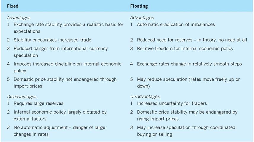
As it has developed since 1973, however, the system has not been one of ‘freely floating’ rates. Instead, governments have tended to intervene from time to time to support the values of their currencies (see Fig. 25.1). For instance, the UK has intervened in recent times to prevent the pound falling when cheap imports were part of its anti-inflationary strategy. The setting, for internal reasons, of particular ‘targets’ for the exchange rate has therefore resulted in a system of ‘managed’ exchange rates, picturesquely described as a ‘dirty floating system’. The major advantages and disadvantages of fixed versus floating exchange rates are shown in Table 25.3.

Sterling and the ERM

In the last 60 years we have moved, as we have noted, from a fixed to a floating exchange rate regime. With the advent of world inflation in the 1970s it became impossible to maintain fixed exchange rate

Table 25.3 Fixed versus floating exchange rates: pros and cons.

parities between countries because internal prices were accelerating at different rates. As world inflation subsided in the 1980s floating exchange rates became less necessary: in addition, the increased volatility of currencies led the major countries to seek some form of greater stability. The countries of the European Community had a particular problem in that it was clearly not possible to create a unified market without fixed parities.

While it has not proved possible to implement any form of fixed exchange rate regime for countries as a whole, the European economies operated an ERM in the period 1979-1999 (see Chapter 27). This pegged currencies to the central unit, known as the ‘ecu’, within a permitted band of divergence. The value of the ‘ecu’ was based on a weighted average of the participating currencies. The ERM of the European Monetary System can now be seen to have been an intermediate step towards the European Monetary Union (EMU) which began its transition phase on 1 January 1999 with the launch of the euro (see Chapter 27).

The UK did not join the ERM when it was estab­lished in 1979, as it was feared that sterling would not be able to maintain its position within the system. After that, when sterling rose as a result of the advent of North Sea oil, it seemed inappropriate to join an exchange rate system where the dominant currency, the mark, was a non-oil currency. After 1987, when the UK signed the Single European Act designed to create the single market by 1993, the question of join­ing the ERM again became a live issue. In fact, before the then Chancellor, Nigel Lawson, resigned in 1989 it was clear that he was attempting to target the value of sterling at DM3 = £1. However, the UK govern­ment expressed a reluctance to join until various conditions were fulfilled. Behind what were clearly political arguments and bargaining positions lay a very real apprehension about the problems which the UK might face on entry. In particular, there was the fear of losing the use of a policy instrument, namely the exchange rate, which might then make it more difficult to use depreciation/devaluation to remedy any trade imbalances with individual countries or the rest of the world. A full discussion of the UK’s entry into, and exit from, the ERM can be found in Chapter 27, and more detail on the operation of EMU can also be found in the chapter.

Key points

■ The exchange rate is usually quoted as the number of units of the domestic currency that are needed to purchase one unit of a foreign currency.

■ Some 66% of transactions in London, the largest centre for foreign exchange trading, are ‘spot’ on any one day, 24% are forward for periods less than one month and a further 10% forward for periods greater than one month.

■ The exchange rate is a key ‘price’, affect­ing the competitiveness of a country’s exporters and producers of import substitutes.

■ A fall (depreciation) in an exchange rate will, other things being equal, make that country’s exports cheaper abroad and imports into that country dearer at home.

■ The Marshall-Lerner elasticity conditions must be fulfilled if a fall in the exchange rate is to improve the balance of pay­ments. Namely the sum of the price elasticities of demand for exports and imports must be greater than one.

■ Because short-term elasticities are lower than long-term elasticities, the initial one to two years after a depreciation may not lead to an improvement in the balance of payments (the so-called ‘J-curve’ effect).

■ The effective exchange rate (EER) for sterling is a weighted average of the six national currencies which are most important in terms of trade with the UK.

■ The real exchange rate (RER) takes account of the nominal exchange rates between the various countries and of the relative inflation rates in those countries.

■ There is increasing concern that exchange rate manipulation is becoming a policy mechanism to achieve balance of pay­ments targets.

■ There is considerable evidence to suggest that some exchange rates are under­valued and others overvalued.

Now try the self-check questions for this chapter on the Companion Website. You will also find useful links to relevant websites.

Notes

1 This analysis assumes that the elasticity of demand for imports is greater than one. In the case of exports, foreign buyers will demand more pounds whatever the elasticity of demand, simply because they are buying more goods as the price in their own currency falls, and the sterling price of exports has not changed.

2 The RNULC are calculated by taking indices of labour costs in the UK and dividing by the weighted geometric average of competitors’ unit labour costs. ‘Normalization’ involves adjusting the basic indices to allow for short­run variations in productivity - so eliminating cyclical variations.

3 During the exchange rate crisis of September 1992, three countries reintroduced exchange controls aimed at reducing the capacity of inter­national banks to borrow in their money mar­kets and then sell the currency for speculative gain. Portugal permitted only between half and one-third of escudos in Lisbon’s money markets physically to be used for currency speculation. Spain demanded that the banks deposit funds interest free for a year to match the amount they plan to sell for foreign exchange. Ireland insisted that the government now take over the management of currency swaps, with the excep­tion of those that are trade related.

References and further reading

Bank of England (2010) Statistics Interactive Database, London.

Benassy-Quere, A. and Coeure, B. (2010) Economic Policy, New York, Oxford University Press.

Buxton, T. and Lintner, V. (1998) Cost competitiveness, the ERM and UK economic policy, in Buxton, T., Chapman, P. and Temple, P. (eds), Britain’s Economic Performance (2nd edn), London, Routledge. Copeland, L. (2008) Exchange Rates and International Finance (5th edn), Harlow, Pearson Education.

Giavazzi, F. and Blanchard, O. (2010) Macroeconomics: A European Perspective, Harlow, Financial Times/Prentice Hall. Goodman, S. (2002) The euro and progress on enlargement, British Economy Survey, 31(2): 31-4.

Jones, R. (2002) The Argentinian crisis - a case study in exchange rate inflexibility and national bankruptcy, British Economy Survey, 31(2): 35-8. Kitson, M. and Michie, J. (1994) Fixed exchange rates and deflation: the ERM and the Gold Standard, Economics and Business Education, 2(Spring): 11-16.

Krugman, P. and Obstfeld, M. (2010), International Economics: Theory and Policy, Harlow, Financial Times/Prentice Hall.

Mercier, P. and Papadia, F. (2011) The Concrete Euro: Implementing Monetary Policy in the Euro Area, Oxford, Oxford University Press.

ONS (2010) UK Balance of Payments - The Pink Book, Various, London, Office for National Statistics.

Sutherland, A. (1998) Why are exchange rates so important?, Economic Review, 16(2).

The Economist (2010) The Big Mac Index. An indigestible problem. Why China needs more expensive burgers, 14 October.

Turner, P. (1997) Britain and the European Monetary System, Economic Review, 14(3). UNDP (2010) Human Development Report 2010: The Real Wealth of Nations: Pathways to Human Development, New York, United Nations Development Programme.

UNCTAD (2010) World Investment Report 2010: Investing in a Low Carbon Economy, New York and Geneva, United Nations Conference on Trade and Development.

Wolf, M. (2010) Balance of payments, foreign exchange reserves and currency implications, Financial Times, 3 November.

World Bank (2010) World Development Report 2010: Development and Climate Change, Washington DC.

The following websites are relevant to this chapter:

ONS Economic Trends: http://www.statistics.gov. uk/statbase/product.asp?vlnk=308

ONS Financial Statistics: http://www.statistics. gov.uk/statbase/product.asp?vlnk=376