INDIVIDUAL AND/OR HOUSEHOLD INCOME AND LIVING STANDARDS: FROM MEASUREMENT ISSUES TO CONCEPTUAL ISSUES AND BACK TO MEASUREMENT ISSUES
How to assess the extent of gender inequality in economic well-being? In rich countries, the most usual indicator of economic well-being is the living standard, a notion based on income.
But in income statistics, many income components are available only for households,[700] not individuals, and living standards—that is, the household income adjusted for the household size and composition—are measured assuming that all incomes are shared within households and are assumed to be equal for all members of a given household. In other words, no inequality can be found between men and women living together in a couple-household, a very frequent situation. Assessing a gender gap in economic resources or well-being on such bases is hardly possible: If incomes are not pooled and fully shared, using household-level information may result in seriously biased estimates of income and living standard inequality. But how seriously? The problem is that not much is known about the actual distribution of income within households. This first section, then, is not so much about gender inequality in income as about the limitations to its measurement, the methodology and conceptualization behind measurement, and the implications for the analysis of gender inequality.That income statistics do not systematically provide individual-level income components is in accordance with the current international standard, following the guidelines defined by the Canberra Group[701] (2001, 2011). Acknowledging that economic wellbeing is more an individual than a collective notion, these guidelines nevertheless refer to the household as the best statistical unit for the production of income statistics, for pragmatic reasons: “The starting unit is the individual, but as individuals typically share income with the other persons with whom they live, most surveys collect information on the income streams of all members of a larger statistical unit, most commonly the household.
[...] A full appraisal of income sharing within a household would require collecting data on the income transfers made within the household which would obviously be very difficult to implement. For these reasons, the choice of the household as the basic data collection unit for collecting income data remains the best compromise” (Canberra Group, 2011, pp. 24-25).In support of pragmatism, one must recognize that it is really very difficult to “distribute” all the income components between individuals. First, some incomes are difficult to attribute precisely to one or another household member—for instance, family benefits or the income from assets owned jointly by spouses. Second, the household members may actually share all or part of their incomes and benefit together from shared assets such as housing; measuring an individual’s income would require knowing the amount of income he/she receives from (or transfers toward) another individual within the household. In addition, living with others results in economies of scale (from sharing a dwelling, equipment, etc.); although this is not, strictly speaking, “income,” it must also be taken into account in the comparison of living standards between individuals. So, except in the case of one-person households, measuring income or living standards at the individual level requires either restricting the notion of income to components that can be precisely attributed to one or another household member or having some knowledge of the extent of income sharing and the distribution of income within households. The same goes for wealth. But knowledge is replaced by two crucial, and distinct, assumptions: that of income pooling and that of equal living standards in the household—as if equality was an automatic consequence of income pooling, while it is an independent assumption. Lack of knowledge replaced by assumptions is the main obstacle to the comparison of income and living standards between individuals in general and between men and women in particular.
This section starts with a brief presentation of the components of household income, focusing on the articulation between categories of incomes and income units and of the standard approach to living standards. Then it turns to the conceptual background, presenting the unitary model of the household and its limits and an overview of other, non- unitary models and of the socioeconomic approach to the financial organization of the household from the perspective of their implications for operational statistical practice. The consequences of lacking knowledge and information at the individual level, especially the consequences for the analysis of gender inequality, are discussed, focusing on the assessment of poverty and the implications of a “unitary” perspective in policies against poverty.
12.2.1 Measuring Income: Components and Units
Household disposable income—that is, the amount a household can spend or save without drawing on its assets—is measured as the sum of all the incomes received in the household over a given period of time net of the sum of social contributions and direct taxes paid by the household and transfers to other households. Three main types of income can be received in a household: income from work/employment, income from property, and transfers, some received from other households (e.g., alimonies, child support) and most received from the state.[702] In this set of components, the primary unit of income is more or less obvious: income from work and employment, including wages, salaries, profits or losses from self-employment, some state transfers related to work (unemployment, sickness and maternity benefits, pensions), some other social benefits such as incapacity benefits or scholarships, and some transfers with other households, such as alimonies, are clearly received by individuals. As for deductions, the social contributions attached to earnings or pensions are “individual,” too. But some other components can be individual or “collective”: for instance, who receives the income from property depends on who the owner is.
Attributing this income to one or another member of the household then requires detailed information on ownership, that is, on who holds the assets or, in the case of joint ownership, the shares held by the different owners. Yet wealth is perhaps even more conceptualized at household level than income; we return to this issue later in the chapter (Section 12.7). Taxation can be joint or separate. Some other components are more “collective,” for instance, family or housing benefits. Of course, none of these doubts arise in the case of one-person households, for which the household and the individual income are the same.Identifying the unit who receives/pays is one thing, but what counts in practice is the level at which the information is available in statistical data sets; by definition, strictly household-level data sets do not provide any information at the individual level. Individual datasets most often provide information limited to earnings (sometimes pensions and social benefits); and data sets providing both individual-level and household-level information do not always detail all the components collected at an individual level.[703] Table 12.1 displays a tentative classification of the components of household income by primary income unit and the level at which they are most often available in large-scale datasets (excluding occasional surveys). It shows clearly that, on the basis of the information available in data sets, employment-related income is the only notion of income that can be easily implemented at the individual level. In consequence, the statistical information on income currently available in most large-scale data sets does not allow one to compute a disposable income at the individual level if the individual does not live alone.
12.2.2 From the Household's Disposable Income to the Standard of Living at the Individual Level: The Statistical Approach
The statistical notion of living standard (or “equivalent income” or “income per consumption unit”) is intended to make comparable the economic well-being of households of different sizes and composition.
Its quality as a proxy for economic well-being is much debated (see also Decancq et al., 2014, Chapter 2, in this volume), but for the time being, it remains the most often used and the basis for the measurement of poverty thresholds (or, in the United States, poverty lines).The standard of living is a construction based on the disposable income (or consumption) of a one-person household taken as a measure of his or her economic well-being. When the household counts more than one person, it is measured so as to take into account the fact that the needs of two (three, etc.) individuals living together are less than twice (three times, etc.) those of one person living alone because of the economies of
Table 12.1 Income components, income units, and availability in statistical data sets
Availability
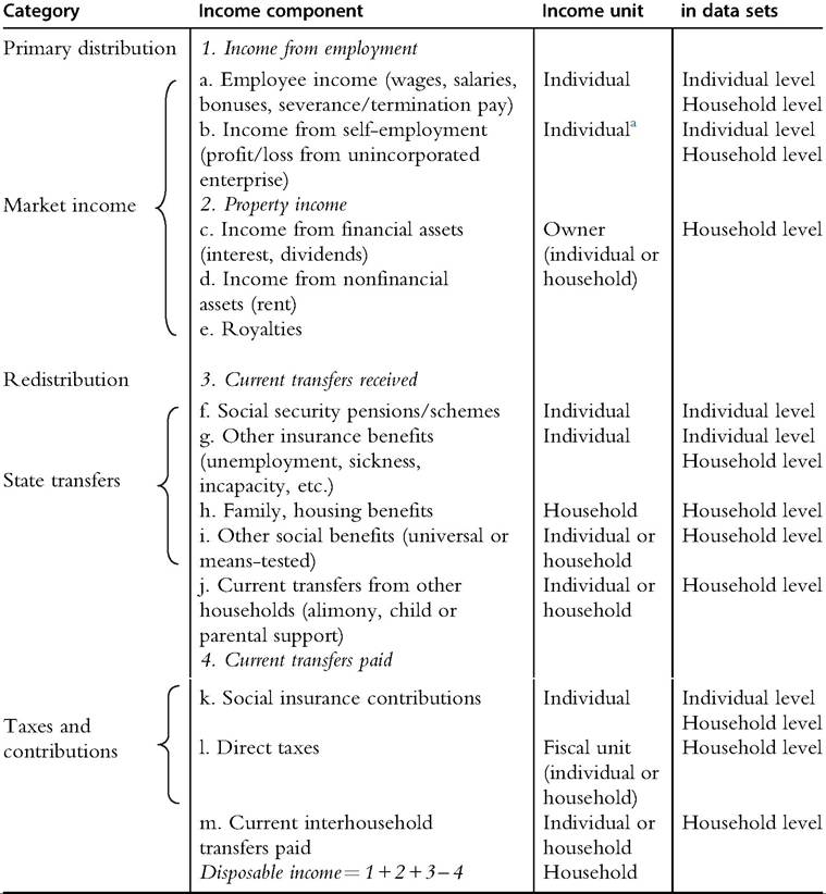
aThe “individual” nature of incomes from self-employment is questionable in the case of a family-ownedbusiness. There are, in general, well-known difficulties in measuring the income from self-employment (see Canberra Group, 2011, pp. 34—35). One particularity is that self-employment income includes income from both employment and capital; the income it yields is generally measured as the amount ofprofit over an accountingperiod (or losses; it can then be negative). Another particularity is that self-employment includes a specific category of employment: “family workers,” who participate in the business of a family member but are not paid.
scale that result from sharing a dwelling and durable and consumption goods and the benefits of the household’s production. The additional income needed to keep the household at the same level of economic well-being when additional members are included in the household is difficult to measure because individuals’ consumption within households is not observed. It is most often estimated on the basis of the observed expenditure of households of different sizes and demographic composition.
These estimations result in “equivalence scales,” which give a weight, assumed to reflect the additional income needed relative to a one-person household, to each additional household member. Whatever the equivalence scale actually implemented, the weight of any additional member is less than 1 (because, as mentioned above, adding a second person to a one-person household does not double the needs of the household). The dominant statistical approach to the standard of living (or equivalent income) currently uses the so-called “OECD-modified” equivalence scale,[704] which gives a weight of 0.5 to an additional adult in the household and a weight of 0.3 to an additional child (a child being an individual younger than 14 years old).While in this section we are more interested in the assumptions behind the measurement of the household’s standard of living and its meaning at the individual level, it is worth briefly illustrating the difference between the household disposable income (INC), a “per head” approach (INCph), and the standard of living, or “equivalent” disposable income (INCeQ). There is, of course, no difference for a one-person household: in this case INCph = INCeq = INC#8725;1. If the household is composed of two adults, then INCph = INC/2 and INCeq = INC#8725;(1 + 0.5); if it is a couple with one child, INCph = INC/3 and INCeq = INC#8725;(1 + 0.5 + 0.3); INCeq is always greater than INCph; the difference accounts for economies of scale. Leaving aside a possible debate on the weightings, it is reasonable (and widely accepted) that INCeq is a better basis than INC or INCph for comparing the level of economic well-being between these three households. But current statistical practice goes a step further, since each individual in a given household is considered to achieve the level of economic well-being he or she would achieve if living alone with an income equal to the household’s equivalent income; in other words, all the household’s members have the same living standard—that of the household. As pointed out by Woolley and Marshall (1994): “The standard approach solves the problem of measuring resource distribution within households by ignoring it” (p. 429). In turn, this practice raises many questions about the actual meaning of indicators at the individual level (including indicators of poverty) based on the household’s equivalent income: if one of the household members holds back some or all of his or her income from the common pool, or if the pooled income is not equally distributed among the household members (or if the equivalence scale does not allow for economies of scale to be “distributed” at individual level; see also Browning et al., 2006a), the approach is much less relevant. This highlights how essential the assumptions of income pooling and equal sharing within the household are both necessary conditions for using equivalence scales (Lise and Seitz, 2011) and deriving individual-level indicators from variables measured at the household level. The standard approach also results in a measure of individual well-being, which, by construction, ignores the possibility of inequality within the household and, by construction, makes intrahousehold inequality virtually impossible to assess.
12.2.3 Behind the Statistical Approach: The Household quot;As Ifquot; an Individual
Curiously enough, the statistical practice of attributing the same living standard to all the individuals living in a household is rooted in a conceptualization of the household “as if’ it was a single individual. The household “as an individual,” first developed in the framework of consumer theory, is the household of the unitary model. This model has many implications for the analysis of gender inequality (Section 12.4); the focus here is on its assumptions and limitations in relation to the practice of income measurement.
12.2.3.1 The Unitary Model of Household Behavior
The unitary model consists in a transposition of individual (consumer) behavior to the household level: according to its preferences, the household maximizes a single utility function under a single budget constraint. For a household to function “as if’ an individual, two main assumptions are needed.
First, individual preferences must converge, one way or another, so that the household can be considered a single decision unit. Considering that the actual agent of the consumer theory is a household (a family), Samuelson (1956) proposed that the family acts as if it were maximizing a joint consensual welfare function, a solution that does not explain the process resulting in a consensus. Another solution to the shift from several individual preferences to a single utility function was provided by Becker (1974a, 1991), proposing that the household is ruled by a “head”—an altruistic or “benevolent” member of the household—who cares about the welfare of the other family members. This would be consistent with the view of marriage based on mutual interest (the gains it provides compared to remaining unmarried) plus love and caring—the addition of optimal associations resulting from the marriage market even making the possibility of shared preferences plausible (Becker, 1973, 1974b). In this approach, the head of household transfers resources to the other household members; the household then acts as a single unit, since the only way the household members can increase their utility is to act in a way that maximizes the utility of the head of household, who in turn will increase his transfers.[705] However, this approach has been shown to hold only under very restrictive conditions (Bergstrom, 1989); a further assumption, which is actually crucial, is also necessary: the altruistic head of household has to be able to control the distribution of resources, meaning either he is richer than the other household members (Ben- Porath, 1982) or he has more power by other means (Folbre, 1986; Pollak, 1985).
Second, the incomes of the household members have to be fully pooled—a necessary condition for there to be only one budget constraint. Income pooling means that the way the income is used (by the household) depends only on the level of the whole/pooled income (and the household’s preferences) and not on the origin of the income.
In the perspective of income measurement, the unitary model then tells us that there is no need to complicate income statistics with information collected at the individual level because it is only the total income of the household, not whose income it is, that counts in the end. However, the head of household does not necessarily treat all the household members equally; then the statistical practice of imputing the same living standard to all the household members may carry the approach a step further.
12.2.3.2 Methodological and Empirical Issues
The unitary model has been challenged on both theoretical and empirical grounds since the 1980s. At the theoretical level, the approach contradicts the methodological principle of individualism at the basis of neoclassical theory (Apps and Rees, 1988; Chiappori, 1992). According to this principle, there is no such thing as “group behavior,” only outcomes from individuals’ decisions. Folbre (1986) also underlines the paradox of “individuals who are entirely selfish in the market (...) [and] entirely ‘selfless’ within the family” (p. 247). The unitary model, along with Becker’s theories on marriage and specialization within the family, also have been much discussed by feminist economists in a general examination of its implications for the analysis of gender (in)equality.[706]
Empirical results do not provide much support. Basically, a test of the unitary model consists of verifying that a change in the distribution of nonlabor income within the household does not modify the structure of the household’s consumption or labor supply behavior (since both are expected to result only from the household’s preferences and the budget constraint, i.e., the pooled income and prices); in short, how the (pooled) income is used should be independent from whose income it is. On the contrary, it has been shown that changes in the personal income level of the partners influence the household’s allocations (Bourguignon et al., 1993; Browning et al., 1994; Phipps and Burton, 1998; Thomas, 1990). Empirical work on developing countries also casts doubt on the validity of the unitary approach (e.g., Kanbur and Haddad, 1994) to the point that, in the mid- 1990s, several economists thought that the time had come “to shift the burden of proof’ onto the unitary model (Alderman et al., 1995). The early results were supported by results obtained from the analysis of the impact of exogenous changes in the household members’ relative incomes, which makes it possible to avoid possible endogeneity biases (for instance, a change in relative incomes resulting from a change in the labor supply). Here, an emblematic study is that of Lundberg et al. (1997); they show that a reform in the payment of family benefits in the United Kingdom—initially paid to fathers, then after the reform to mothers—resulted in an increase in household expenditure on children’s clothes, a result not consistent with the unitary model.[707] Such conditions of “natural experiments” (more precisely, changes that exogenously redistribute the incomes within households) are difficult to find, and comparable studies do not exist for rich countries.[708] However, considering the results of empirical studies over a period running from 1994 to 2008 in different contexts and for outcomes as different as, for example, labor supply, children’s health, savings, demand for clothes, and demand for alcohol and tobacco, Browning et al. (2011) concluded that: “the evidence seems overwhelming: a principal implication of the unitary model is rejected on a wide set of data sets for a wide range of outcomes” (p. 225).
12.2.4 Other Representations of the Household
Several other nonunitary models of household economic behavior have developed since the early 1980s. Parallel with these developments, a strand of research in sociology and economic psychology examines the financial organization of the household. We now look at these alternative economic models[709] and socioeconomic approaches and the alternatives for statistical practice they offer.
12.2.4.1 Nonunitary Models of the Household
Contrary to the unitary model, nonunitary models explicitly consider the individuals within the household in accordance with the methodological principle of individualism, and they take into account a notion of relative power in decision making, allowing for a gendered approach to intrahousehold organization. Nonunitary models generally consider two decision makers (spouses), each with his or her own utility function,[710] allowing for externalities—that is, including the partner’s preferences in their utility functions. The partners’ relative power in the decision-making process is taken into account either as the utility each partner would obtain outside the marriage or in a sharing rule. Two categories of goods are considered: private goods, corresponding to goods that can be consumed only by one partner (and will be included only in one partner’s utility function), and public goods that can be consumed at the same time by both partners. Children do not directly influence household decisions, but their well-being is taken into account as a public good in the parents’ preferences. Incomes are not necessarily assumed to be pooled (but they can be), and the origin of income contributes to the partners’ relative power, as well as various other distribution factors, that is, factors that may influence the decision process but do not change the budget constraint: typically the partners’ nonlabor incomes, education levels, health status, wealth, or social capital. The distribution factors can also be external to the partners’ characteristics: the state of the labor market or the marriage market may shift the power balance through the opportunities they offer outside the partnership. Folbre (1997) also refers to “gender-specific environmental parameters” such as women’s rights in general, marriage and divorce laws, and property rights. Agarwal (1997) extends the understanding to the influence that this environment, including social norms, can have on the actual scope for bargaining within the household.
Beyond these broad characteristics, nonunitary models differ in the assumptions made about whether decisions result in Pareto-efficient outcomes—that is, when improving one partner’s well-being is not possible without reducing the other’s—and in the way they represent the process of decision. There are three main categories of nonunitary models: cooperative bargaining models (Manser and Brown, 1980; McElroy and Horney, 1981), noncooperative bargaining models (Ulph, 1988; Woolley, 1988), and collective models (Bourguignon and Chiappori, 1992; Browning et al., 1994; Chiappori, 1988). Drawing on game theory, bargaining models have in common the assumption of a certain process of decision making but not necessarily that the outcome is Pareto-efficient; on the contrary, collective models do not specify a particular decisionmaking process but assume Pareto-efficiency, justified by the stability of the relationship (see more detailed presentations in Chiappori and Meghir, 2014, Chapter 16; Browning et al., 2006b; Donni and Chiappori, 2011). However, Pareto-efficiency becomes difficult to assume when the household’s environment is not stable, for example, when decisions change the partners’ relative bargaining power or if what seem to be optimal in a given context can lead to nonoptimal outcomes when the context is changed. The exploration of these dynamic aspects is one of the directions taken by most recent research (e.g., Basu, 2006; see also Chiappori and Meghir, 2014, Chapter 16).
Bargaining models have introduced the notion of “threat point”; the basic idea is that neither partner would agree on a decision resulting in a lower level of individual utility than that he or she could achieve if the partners did not come to an agreement. The individual level of utility (the utility at the threat point) defines a partner’s bargaining power. The threat point was formulated first as a divorce threat—a rather radical argument of negotiation, as underlined by Bergstrom (1996). Another formulation is that of the model of “separate spheres” (Lundberg and Pollak, 1993); here, the threat is not defined in terms of union dissolution but as minimal cooperation, with each partner being responsible for a given sphere (defined by social gender norms) of common consumption.12,13 The interest of the bargaining approach is to provide a framework for analyzing unequal power relations within the household and how they can be influenced by environmental factors. Folbre (1986) emphasizes the importance of this difference from the unitary model: “It is the juxtaposition of women’s lack of economic power with the unequal allocation of household resources that lends the bargaining power approach much of its persuasive appeal” (p. 251). However, these models present serious difficulties of estimation, especially the need to identify a threat point, as described by Himmelweit et al. (2013).
Because they do not refer to a specific decision process, collective models do not face this particular problem. They can be seen as a general class of cooperative models and are nowadays the dominant approach to household decision making. In these models, the partners maximize a household utility function, which can be seen as a weighted average of each partner’s utility function; the weighting corresponds to a sharing rule, which depends on distributional factors and reflects the partners’ relative power (instead of “points” where marriage or cooperation breaks down). Empirical results regularly show that the sharing rule is influenced, as expected, by various characteristics of the household members and contextual parameters (Browning et al., 2011). Empirical applications, however, often require more assumptions because neither the outcome nor the sharing rule are observable and statistical information is most often available only at household
12 The difference from the external threat, where the bargaining power depends on the utility the partners would get outside the partnership, is that in Lunderg and Pollak’s (1993) setting it depends on the resources the partners bring to the marriage. These two views of the threat point may lead to completely opposite policy implications.
13 Other models that are not detailed here introduce the possibility of transfers between partners (Carter and Katz, 1993; Chen and Woolley, 2001) or specify several threat points (Bergstrom, 1996). level. In addition, while variations in the sharing rule can be estimated, it is much more complicated to obtain estimations of the sharing rule itself[711] (Himmelweit et al., 2013).
Nonunitary models provide a conceptual alternative to the unitary approach and have allowed many improvements in the analysis of the household members’ behavior within the household, but, in the perspective of statistical practice, they do not provide the operational alternatives that would allow going beyond the convenient assumptions of the unitary ground, in part because their estimation requires additional assumptions that reduce their scope and in part because of the lack of large-scale individual data on income.
12.2.4.2 Intrahousehold Finances: A Socioeconomic Perspective on Income in the Household
In sociology and economic psychology, the household (actually the couple-household, as in most economic models) is analyzed as a place ofbargaining between partners of unequal power and may have conflicting interests. The household’s domestic organization is explained within the main framework of the theory of resource exchange, which predicts that the partner with the highest resources—income, education, status—will have more power within the household (Blood and Wolfe, 1960; Sabatelli and Shehan, 1993). The notion of resources may include opportunities outside the relationship and the costs of an exit solution—an idea interestingly close to that of economic nonunitary models.
The issue of intrahousehold distribution of income is addressed in terms of financial organization, characterized by the management of and control over money by the partners. Another notion, not present in economics, is that of different categories of money— or “monies,” according to the term introduced by Zelizer (1989, 1994)—depending on whose money it is and linking it to specific uses, some of which are shaped by gender norms: as in the case of labor division, money management reveals gendered relations ofpower (Tichenor, 1999). “Money” is not “income,” but the questions addressed about money in the household are strikingly similar to those addressed in economics about the distribution of income within the household: Does the origin of money matter? Is it possible to lack money in a rich household? Who has power over what money? Who is responsible for given expenditures? Who makes decisions about what?
A very influential classification of money management systems, intended to reflect gradations of control over money, was proposed by Pahl (1983, 1989). She defined four main systems.[712] (1) The “whole wage” system: one partner hands over all his or her wage (minus an amount of “pocket money”) to the other, who is in charge of managing the household’s finance; this other partner may or may not have a personal income. (2) The “housekeeping allowance” system: here, one partner hands over an amount to be used for housekeeping spending and manages the rest him/herself.In these first two systems, only one partner has control over the household money. (3) The “pooling” or shared system: both partners manage and use the money as they need either for common or personal expenditure. (4) The “independent management” system: each partner keeps separate control over their income; unlike the three other systems, there is no notion of household money and neither partner has access to the other’s money. This classification has been central in many dedicated studies of quantitative sociology and socioeconomics over the 1990s (e.g., Burgoyne, 1990; Burgoyne and Morison, 1997; Treas, 1993; Vogler, 1998) and remains the reference in recent empirical work (see Bennett, 2013).
One of the interests of Pahl’s classification is that it provides usable survey questions[713]: typically, the respondents are asked whether they pool all, some, or none of the income, and sometimes the share of their income they pay into a “common pot” or the share they spend on their own private consumption.[714] Empirical work generally finds that the pooled system is more often observed in the case of married couples (Heimdal and Houseknecht, 2003; Ludwig-Mayerhofer et al., 2006; Lyngstad et al., 2011), couples who have children (Hamplova and Le Bourdais, 2009; Kenney, 2006; Laporte and Schellenberg, 2011; Vogler et al., 2008), in one-earner families or when the income imbalance is significant (Elizabeth, 2001; Hallerod, 2005), and when money is tight. It is less frequent when the partners have higher education levels (Laporte and Schellenberg, 2011), in the case of past partnerships, or when there are financial ties with other households (Burgoyne and Morison, 1997; Heimdal and Houseknecht, 2003; Treas, 1993). In summary, bearing in mind that different methodological options[715] and data limitations sometimes make the results difficult to compare, duration, the presence of public goods (especially children), a traditional division of labor, and the need to monitor low resources seem to have a positive influence on the probability of pooling incomes. Beyond this general pattern, comparative studies show significant cross-country variation that might relate to different institutional and cultural contexts (Hamplova and Le Bourdais, 2009; Heikel et al., 2010; Heimdal and Houseknecht, 2003; Yodanis and Lauer, 2007). As for the overall incidence of the pooled system, the main result is that significant proportions of couples declare that they keep at least some of their money separate,19 another dent in the unitary model insofar as the concept is the same as that of income pooling in the economic literature.
From the perspective of statistics appropriate for the study of income inequality between individuals, implementing “pooling” questions on a systematic basis has some appeal. It would be an easy way to determine whether incomes are fully pooled. If so, this would justify a unitary approach; if not, some additional questions on the share of different incomes held back from the “common pot” by the household members would make it possible to estimate the amount of income actually available to, or controlled by, each member. However, several questions can be raised. One is what is actually captured by the answers to pooling questions: a perception of more or less collective money, a practice of management, or actual control over one’s own or the household’s money? It is also difficult to deduce whether there is equality within the household from the pooling regime. Transfers between partners can take place without income pooling, and hence no pooling does not mean no sharing; conversely, income pooling does not necessarily entail equal or fair sharing. Another issue is how the respondents understand the income/ money questions: contrary to in-depth interviews, where the researcher can interact with the respondent to ensure a common understanding, survey questions may be understood differently from their intended meaning. Finally, there is the question of the identity of the respondent: is it a unique respondent, representative of the household, or both partners? Questions asked of only one partner may provide reductive information, but asking both partners may lead to dealing with conflicting answers.20,21 Beyond “technical” questions, the pertinence of the information obtained from survey questions on the pooling regime is questioned in qualitative research. For instance, exploring the case of partial pooling and separate finances, Ashby and Burgoyne (2008) suggest that they may conceal more complex practices relating to perceived ownership and commitment in the
19 A presentation of the main results of the EU-SILC 2010 module on “Intra-household allocation of resources” shows that, among the 27 EU member states, about 70% of the households (with at least two adults)—ranging from as low as 50% in Austria to about 85% in Malta—reported that all the incomes are treated as common (Eurostat, 2012).
20 In an analysis of individual or household responses to questions on perceived economic well-being, Plug and Van Praag (1998) found that, when asked about the minimum income needed to maintain a family like their own, there was no difference between the partners’ responses in one-earner and two-earner couples, as long as the earnings differential was not substantial.
21 The analysis of the Eurostat module on intrahousehold sharing of resources (EU-SILC, 2010) shows that there are significant proportions of households in which the partners’ responses are not coherent, as well as of “full pooling” households in which at least one partner reports that they keep some of their own income from the pool (Ponthieux, 2013).
relationship, and hence do not provide accurate insights into the partners’ living standards or control over money.
Another issue is whether the pooled system actually corresponds to the income pooling assumption. The few studies that have addressed this question seem inconclusive: Bonke and Uldall-Poulsen (2007) found a high correlation between the “pooled system” and an experiment-type measure based on answers to a question asking whether the respondents would spend more or less on themselves if their own and their partner’s incomes were changed in opposite directions; partners using a pooled system were more likely not to change their personal spending. This result suggests that the two approaches correspond to the same notion. But Bonke (2013), using the same data set (the Danish expenditure survey) and questions allowing the household’s consumption over a large set of goods to be assigned, finds that the structure of the household’s expenditure seems to be correlated with the income distribution, even in households having reported a pooled system. In that case, the pooled system would not correspond to the assumption of income pooling.
12.2.5 Back to Measurement and the Pending Question of Intrahousehold Distribution of Income: Where We Stand, the Consequences, and Gendering the Issue
Concern about the distribution of income within the household is not new; in 1952, an article on “The distribution of income within the family” (Young, 1952) started as follows: “It is painfully obvious to the student of social policy that growing knowledge about the distribution of the national income between families has not so far been matched by a growth in knowledge about the distribution of the family income between its members. In place of knowledge, the assumption has often been made, though not stated, that the family... can still be treated as a unit for the purposes of spending. It has been taken for granted that some members of a family cannot be rich while others are poor.... To replace assumption by information is no small venture” (p. 305). More than 60 years later, it is painfully obvious that statistics on income and economic wellbeing remain based on the unitary version of the household,[716] as if stuck in a conceptualization now widely considered inappropriate. The gap between research and statistical practice has simply increased over time.
Statisticians are not unaware of the problem when deriving indicators of inequality between individuals from variables at household level. Although it is acknowledged that, in principle, the unit of interest is the individual, the argument that because incomes are shared the pertinent unit of collection is the household still holds[717] (Canberra Group, 2011, p. 24) or that, in doubt, it is preferable to assume that incomes are shared rather than the contrary (Forster and Mira d’Ercole, 2009, p. 7). So, at present, how to get a better idea of inequality in living standards within households remains an open issue. Taking a step forward in the conception of income data would entail a shift from household-level data to data systematically providing individual-level information on income components received or transfers made by and to individuals. There would, of course, be a cost in terms of data collection, and this would not in itself solve the question of the actual extent of sharing within households; but being able to use information disaggregated as much as possible would give more flexibility to testing various assumptions about income pooling and sharing and would allow escape from a situation in which the measurement of individual economic well-being and the analysis of inequality between individuals is conditioned in the first place by the assumption that individuals are equal within the household in which they are observed.
12.2.5.1 “How Serious Is the Neglect of Intrahousehold Inequality?quot;[718]
One major difficulty in assessing the potential consequences of ignoring inequality within households is, ironically, the lack of data on individual income. It is nevertheless possible to illustrate what the standard approach ignores when attributing an equal standard of living to each member of a household. We draw here on the framework proposed by Jenkins (1991, pp. 476-477). For a couple-household, a simplified formulation of the living standard (Eq-Y), taken as the household budget constraint, defines it as the sum of each partner’s earnings plus the couple’s net nonlabor incomes (NL) divided by the number of equivalent adults (neq) to account for the economies of scale[719]:
Gender Inequality 1001
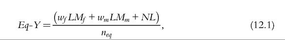
where w is the earnings rate, LM the time in the labor market, andf and m identify females and males, respectively.
The standard approach assumes that Eq-Yf = Eq-Ym. This implies that any difference between wfLMf and wmLMm is counterbalanced by implicit transfers between the partners and that NL is received jointly or equally shared, and it assumes that the economies of scale are distributed equally between the partners. To take into account other neglected possibilities, the couple’s total income, including the economies of scale (assumed separable), can be rewritten as
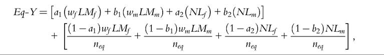
where the first part of the right-hand side corresponds to the amount of incomes not pooled, and the ais and bis represent the share of income each partner holds back from the pool.
This amount illustrates the potential ignored inequality within a couple-household; it involves the degree of inequality between the partners’ earnings, whether nonlabor incomes are received jointly or separately (which, in the case of capital income, raises the issue of asset ownership within multiperson households), and, of course, the share of his or her incomes each partner holds back from the pool. Whether this share is large or small remains unknown. However, the “pooling question” of the European survey “Intra-household allocation of resources” (EU Statistics on Income and Living Conditions [SILC] ad hoc module 2010) provides an order of magnitude of the proportions of individuals and households for which this share is not 0: over 21 European countries, the mean percentage of adults living in multiperson households who reported holding back at least some of their income from the pool was about 47%. At a household level and including one-person households (for which the assumption of full pooling is always true), this yields 38% of all the households in which at least one household member does not pool all his or her income (Ponthieux, 2013). Even though caution is necessary when interpreting the “pooling question” (see Section 12.2.4.2), this suggests a rather high risk of assuming full pooling when it could be unjustified. The next issue is that of the impact this may have on the measurement of economic inequality between men and women.
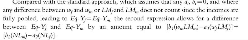
In the 1990s, several studies explored how men’s and women’s poverty rates would differ from the conventional measures under assumptions other than intrahousehold equality (Borooah and McKee, 1993; Davies and Joshi, 1994; Findlay and Wright, 1996; Fritzell, 1999; Phipps and Burton, 1995). The most general principle consists of applying an “unequal” distribution of income instead of the equal distribution assumed by the standard assumption; the “individual” income is then computed as if only the household nonlabor income was shared, using various assumptions about how it is distributed.[720] Whatever the year, country, or methodology, all these studies find that departing from the standard assumptions results in increased gender gaps in poverty (Table 12.2). In the case of married men and women, income poverty rates are dramatically higher for women and significantly reduced for men, instead of the equal poverty rates obtained with the conventional approach; when all households are included, the changes are less pronounced, mitigated by the relative share of one-person households for which the assumption has no effect.
Sutherland (1997) computed individual incomes assuming that all income is retained by the person who receives it, that the collective components of income are received by the head of household, and that family benefits are received by mothers—to whom Sutherland also allocates the responsibility for children. She shows that women are disproportionately represented in the bottom quantiles of the distribution of individual incomes, contrary to broadly equal shares of men and women in each quantile of the distribution of household income. A more recent study by Meulders and O’Dorchai (2010) suggested that the gap between conventional measures based on household incomes or “individual” incomes remains substantial. Using harmonized European data (EU-SILC) from 2006 for nine countries, they computed individualized incomes as the sum of the incomes received individually by adult men and women and, for those living in multiperson households, an equal share of the income components available only at the household level.[721] Then they compute a threshold at 60% of the median individual
| Table 12.2 Sharing assumptions and poverty risks by gender Sharing assumption Authors, country, year, population | Equal sharing of household income | Other assumption on sharing | ||
| Men | Women | Men | Women | |
| Women get 30% of the couple's market income Borooah and McKee (1993), United Kingdom, 1985, married couples % below 2/3 mean equivalent income | 33 | 33 | 14 | 66 |
| Each adult keeps her/his own incomea Phipps andBurton (1995), Canada, 1986, married couples % below 50% median equivalent disposable income | 10.5 | 10.5 | 4.5 | 28 |
| Each adult keeps her or his own incomea Davies andJoshi (1994), United Kingdom, 1986, married couples % below 20th percentile equivalent disposable income | 15 | 15 | 11 | 52 |
| Women get 20% less than their equivalent incomea Findlay and Wright (1996), United States, 1985; Italy, 1986; all adults % below 50% median equivalent disposable income Italy | 17.5 | 16.8 | 15.4 | 27.1 |
| United States | 17.0 | 22.6 | 15.9 | 30.3 |
| No sharinga Fritzell (1999), Sweden, 1991, adults aged under 65 % below 50% median equivalent disposable income | 4 | 3.9 | 4.5 | 9.6 |
aThe authors also present other assumptions or computations for other household demographic compositions than those reported in this table.
income and measure the risk individuals would face of falling below this threshold (called “financial dependency”) if they lived only on their own financial resources.[722] The comparison of the two approaches shows that the conventional methodology has much more influence on women than men: over the nine countries, men’s ratio of “financial dependency rate” to poverty rate ranges from 0.7 to 1.4 and women’s changes from 1.7 to 3.3.
These results seem convincing enough to answer the question in the heading above: yes, neglecting intrahousehold inequality can be serious.[723] But while they show clearly that assumptions matter, it is more difficult to draw conclusions in terms of individual living standards; the main conclusion is that the living standard is a household-level notion and that household-level information fails to inform about individual situations within households.
12.2.5.2 The Standard Assumptions and the Assessment of Gender Economic Inequality
As exemplified above, by construction, the standard assumption of equality within households puts serious limits on the assessment of the extent of gender inequality. The crux of the problem is that the household dimension comes up entangled with individual characteristics, not only making an overall assessment of gender economic inequality virtually impossible but also obscuring the causal factors of gender inequality behind the household dimension. This is not to say that the household dimension has no effect on men’s and women’s economic outcomes—it certainly has strong effects, as will be obvious in the next sections—but the conventional measure of economic well-being conflates individuals and households, making individual situations intractable. The analytical challenge is to disentangle individual outcomes from household outcomes to understand how the “household dimension” both contributes to (because of decisions made in the household context) and obscures (because of assumptions about the absence of inequality within the household) gender inequality. This understanding may, in turn, have various implications in the perspective of public policies aimed at reducing inequalities.
The comparison of individual labor market status and outcomes and the risk of poverty is especially illuminating: in the working-age population, women, despite their lower participation in the labor market (see Section 12.3) and their disproportionate presence among low-wage workers when they do work (see, e.g., Grimshaw, 2011), do not face dramatically higher poverty rates than men: the gap (women—men) ranges from 2.2% to 2.9% points in English-speaking countries, between 0.9 and 2.1 in continental and southern European countries, and is negative in Nordic countries (figures are from Table 1 in Gornick and Jantii, 2010[724]). Moreover, Gornick and Jantii show that, among individuals of working age with low or no earnings, women are less likely to be poor than men. In a study including 22 EU countries, Maitre et al. (2012) found the same pattern among low-paid workers: men’s poverty risk is notably higher than women’s. A similar “gender paradox” is underlined in empirical studies ofthe working poor (Peiia-Casas and Ghailani, 2011; Ponthieux, 2010). This, of course, has a lot to do with the fact that in the working-age population, a large proportion of men and women live in couple households, a configuration in which there is no inequality by construction. The measure of women’s economic well-being then seems to be much less related to the outcome of their individual economic activity than men’s. However, this is precisely because their earnings are, on average, lower than men’s. Because of this inequality and the large share of adults who do not live alone, the influence of the equal sharing assumption is the greatest on the estimates of women’s poverty rates.
What does this imply in terms of public policies? Many social transfers target the households (families, fiscal units) and assess their efficiency on the basis of outcomes measured at the household level. The implicit assumption is that meeting the needs of individuals is achieved by meeting the needs of households—another formulation of the unitary model. It is the same when individual benefits are conditioned by household resources, implicitly assuming that there cannot be needy individuals in nonneedy households. How this may affect the economic well-being of the individuals within households is, by construction, difficult to assess precisely because conventional measures of economic well-being and policy targets are derived from household-level information. While no statistical information allows for an assessment of the incidence of individual poverty in nonpoor, multiperson households, there are reasons to believe that neglecting the intrahousehold distribution of resources can contribute to the persistence of gender inequality. Policies that link what an individual is entitled to with the actions or resources of another member of his or her household can reinforce the imbalance of resources between men and women and women’s economic dependence.
However, even accepting that intrahousehold transfers are such that equal living standards are achieved despite unequal personal resources, and that, contrary to what empirical results suggest, the imbalance of resources within households is not an issue, the equilibrium can be fragile. The trend of decreasing marriage in favor of cohabitation and increasing divorce or separation rates results in an increase in the number and types of households an individual may belong to over his or her life cycle. This suggests that resorting to household outcomes to assess individual situations may become increasingly irrelevant. From the perspective of measuring and analyzing gender inequality, this calls for a change of framework; as long as women’s labor market outcomes are less favorable than men’s, as is still the case, the standard approach, bypassing the issue of intrahousehold inequality, conceals gender asymmetries in the relation between the market and the household and inequality in terms of autonomy, risks, and opportunities.
12.3.