INEQUALITY OF OPPORTUNITY: MEASUREMENT ISSUES AND EMPIRICAL RESULTS

This section will focus on methodological issues and applications of the theory. An excel­lent survey of the material covered in this section is provided in Ramos and Van de gaer (2012).^[154]

4.10.1 Methodological Issues: General Remarks

We begin with some general remarks for the reader who is familiar with the literature on the measurement of inequality of outcomes.

32

4.10.1.1 EOp Measurement as a Multidimensional Problem

Nevertheless, it seems fair to say that the level of complexity of the analysis is greater because EOp is multidimensional. Equality-of-opportunity analysis may use the concep­tual framework developed by Atkinson and Bourguignon (1987) in the field of multi­dimensional inequality. These authors focus on how to measure income inequality when each income unit belongs to a specific needs group. The information is two- dimensional—income and needs for each household—and the aim of the analysis is to rank income distributions taking into account the information provided by the vector of needs.

A direct application of the sequential Lorenz quasi-ordering to this setting is not appropriate and it is interesting to see why. Of course, effort can be seen as analytically similar to needs; that is, at the margin, the more effort one expends, the more one deserves. Reciprocally, circumstances can be seen as negative needs: the better one’s cir­cumstances are the less one deserves. But these two statements have limitations. We may wish not to reward effort excessively, for reasons discussed in Section 4.4. And regarding circumstances, there is an asymmetry: we desire to compensate for disadvantageous cir­cumstances, but do not regard advantaged circumstances as an evil. Furthermore it is the interplay between circumstances and effort that makes the evaluation of the ensuing inequality problematic. We need to know how additional effort should be rewarded across the circumstance dimension; as we discussed, there is no clear answer to this ques­tion within the theory. For further discussion, see Bossert (1995), Fleurbaey (1995), and Fleurbaey and Peragine (2013).

4.10.1.2 EOp as a Process

What also distinguishes EOp empirical analysis from inequality-of-outcome analysis is its two-stage nature: one generally requires an econometric-estimation stage, preceding the inequality-measurement stage. It is not so much the difference in circumstances per se that matters, but the difference in the impact of circumstances.

In principle, we agree. This is, however, more easily said than done. Two observa­tions are in order. The two main obstacles to any causal inquiry are reverse causality and endogeneity due to omitted variables. The good news is that, regarding circumstances, reverse causality can often be dismissed since circumstances are frequently characteristics of states that existed in the past (e.g., one’s parents’ education). However, endogeneity cannot be discarded in that way since EOp measurement is plagued with informational problems. Omitted variables are widespread; a good example is provided by genetic vari­ables which have been found paramount in income attainment by Bjorklund et al. (2012). Omitted variables in empirical EOp analysis cause skepticism in claims of causality we may wish to assert. The situation is even worse when the objective is earnings, since according to Bourguignon et al. (2007), “an instrumental variable strategy is unlikely to succeed, since it is difficult to conceive of correlates of the circumstance variables that would not themselves have any direct influence on earnings.” Experiments and quasi­experiments enable one to make causal statements, but experiments can usually only study problems which are much more circumscribed than those which interest researchers in this field. We are trying to understand the whole process by which some­one reaches an income level, a health status, or an educational attainment.

Should we worry about this lack of causal interpretation? Of course, if we want to give advice to policy makers about the true effect of level-the-playing-field policies, impact evaluation needs to be causal. However, if one merely wants to measure the degree of inequality of opportunity—that is inequality due to circumstances—a correla­tion (with variables which occurred in the past) is already something that is relevant.

The challenge is even greater if we use the preference view for responsibility variables advocated by Dworkin and Fleurbaey. Retrieving the true parameter of the preferences is perhaps the most difficult issue in econometrics in terms of identification conditions. See, however, Fleurbaey et al. (2013) for an attempt to estimate the individual’s trade-off between health and income and Bargain et al. (2013) for the estimation of cross-country preference heterogeneity in the consumption-leisure trade-off.

4.10.1.3 Lack of Relevant Information

It should be clear from this discussion that we need a much richer database to perform EOp empirical analysis than a pure inequality-of-outcome analysis. We should have variables describing the situation of the family and social background and variables per­taining to effort. It is quite common that some important background variables are missing and then we have an incomplete description of the circumstances. More importantly, effort variables are generally missing for the very reason that effort is pri­vate information, as is emphasized in economic theory. We must use proxies, which are problematical.

The measurement of effort depends on our view of responsibility. On the one hand, there is the view that effort takes into account what set of actions a person can access, where access is a question not simply of physical constraints, but of psychological ones, which may be determined by one’s circumstances.

Several points that should be made about two variables that appear repeatedly in empirical analysis when trying to measure EOp in income attainment: the number of hours of work and years of education. The number of hours of work is a good effort variable, under the control view, for self-employed occupations, but is clearly less satis­factory for wage earners. It is true that hours of work correspond to a quantum of effort: The issue is whether they correspond to the desired amount of hours. Part-time jobs may be involuntary; overtime work may depend on the orders of the firm, and obviously unemployment may be just bad luck. Toa large extent, using hours of work in a given period as an effort variable is therefore problematical for wage earners. We can be more confident that the number of hours of work over the life span is under the control of the individual because one can compensate for the impact of bad luck and low hours of work during a given period by working more in luckier periods.

33

Years of education is also a popular effort variable in empirical studies. It is contro­versial to consider it as a variable under individual control, because primary and secondary education take place when the person is a child and adolescent, largely prior to the rel­evant age of consent. If a child is lazy in school, there might be factors not under his con­trol that explain his laziness. Only tertiary education and lifelong learning are immune from this criticism. The problem with tertiary education comes from its path­dependency: One’s probability of being accepted to university depends on one’s grades in secondary education, which, in turn, depend on achievements in primary school. The above-mentioned problem for the two early stages of education then contaminates higher education attainment.

A good starting point is to attempt to account for achievements in early education by circumstances of the family. Socioeconomic circumstances may be available in data sets, but parental pressure to achieve is also an important determinant of educational out­comes, and is usually not measured. We cannot, therefore, usually give a complete account of educational achievement. However, if one views all actions of the child as due to either nature or nurture, both of which are beyond his or her control, by hypoth­esis, before the age of consent, then one should simply take the child’s educational accomplishments at the age of consent as a circumstance with respect to determining out­comes in later life. Family circumstances may still be important in explaining choices after the age of consent: for example, a young adult might not attend college both because his achievements in secondary school were mediocre (which, according to the view just expressed would be a circumstance) and also because his parents put little value on tertiary education (also a circumstance). Facing these two circumstances, if a low-achieving 18-year-old nevertheless succeeds in going to college, through taking compensatory courses, that would be ascribed to exceptional effort, ceteris paribus.

In both the hours of work and education examples, then, we will often not have an accurate measure of effort. It will be measured with error and bias. Broadly speaking, the authors do not pay sufficient attention to these problems and overlook their prac­tical implications. Since effort measurement does not have the same robustness as cir­cumstance measurement, choosing effort as the conditioning variable as in the tranche approach (see for instance, Peragine, 2004; Peragine and Serlenga, 2008) seems risky. True, circumstances may be only partially described, but generally they are not noisy. Since tranche and type approaches seem incompatible (see below), conditioning on type seems a better choice than conditioning on tranches for a measurement error problem.

4.10.1.4 AgeandSex

The issue of availability of information cannot be raised about age and sex. The problem is how to treat these variables. Under the control view, age and sex are circumstances. Under the preference view, because age and sex are important determinants of prefer­ence, they will implicitly enter as factors of effort. Because, under this view, preferences should be respected whatever they are unless they are not well-informed, they are put on the responsibility side of the cut.^[156] Of course, as Fleurbaey and Schokkaert (2009) pointed out, we are free, once the true impact of age and sex has been identified econo- metrically, to test whether it matters to put age and sex on one side or on the other (see Garcia-Gomez et al., 2012 for an application). When we are explaining health, it does not come as a surprise to learn that 45% of the explained variance in health comes from these two demographic variables (seeJusot et al., 2013). This is not the thorniest issue in EOp measurement, but the reader should be aware that the extent of inequality of opportunity may depend on whether or not one includes these variables in the responsibility set. For instance, Almas et al. (2011) put age among the responsibility variables, on the ground that our concern should be with inequality of lifetime earnings. Another solution would be to exit the dual world of the model and to admit that there are variables that are neither under the control of the individual nor for which compensation is due. An example is provided in the health sphere where it is admitted, by most, that health policies cannot erase the impact of demographics. (We should not consider males disadvantaged with respect to females if, due to innate biological factors, their life expectancy is shorter.) For earnings achievement, this stance cannot be easily argued, because differences in returns, linked to gender and perhaps age, may be related to discrimination, which would obviously be a violation ofEOp.

As in other domains of econometrics, there is a large issue of what to do with poor data. The mistake to avoid is pretending that a poor data set is rich. Innovative methods exist to deal with missing variables. An important methodological issue that has been raised and partially solved is to deduce what can be said about inequality of opportunity when we know that the observables are far from recovering the process through which the objective has been attained. We should adapt our empirical strategy to the richness of the informational structure ofthe database. Basically, we can contrast situations from the richest informational setting to the poorest one. In the first situation, we have a good description of the world, that is, a quite comprehensive set of circumstances and some candidates for effort variables. In the second situation, no effort variables are available and individuals can be ranked in broad type categories. We will contrast the methods accordingly.

34

4.10.2 The Estimation Phase

4.10.2.1 The Case of a Rich Data Set

The first choice is to decide between parametric and nonparametric estimation. Because, by assumption, there are many observable variables, a parametric estimation will fit the data better (see, Pistolesi, 2009 for a semiparametric estimation). Bourguignon et al. (2007) took the lead regarding the econometric strategy in this case. We should estimate a system of simultaneous equations. The first equation will describe the process of attain­ment of the outcome. In the income context, it can be called a return equation, the coef­ficient of each determinant giving the marginal return (in a linear model) of each determinant whether it is a circumstance, effort, or demographic variable. The other equations (one for every effort variable) will relate the effort variable to circumstances and other control variables. In the control view of responsibility variables, we should understand how variables that are outside the control of the individual influence her effort variables. In these “reaction equations” circumstances must be introduced, includ­ing market conditions (prices, any market disequilibrium such as the local rate ofunem- ployment for job decisions), and demographics. One supposes that the reaction of individuals to their environments (market and background conditions) may vary across individuals. We should let the coefficients vary according to demographics. The differ­ence in the value of these coefficients, if any, would be interpreted in a different way according to the control versus the preference view. According to the latter, they are preference shifters, whereas according to the former they are driven by circumstances, and belong to the nonresponsibility side of the cut.

We introduce some notation. Let y_i be the outcome of individual i (the original out­come variable or some function of it), C_i the vector of circumstances, E_i = (e_i1,...,e_ij,..., e_ik) the vector of effort of dimension k, D_i the vector of demographics, M_i the market conditions prevailing for i, ε_i, the mean-zero residual of the return equation, and o_ij the mean-zero residual of the reaction equation of effort j. The other letters employed are for coefficients of both regressions. In the simplest linear model the following equa­tions have to be estimated:

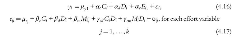
Equation (4.16) is written in a compact way: Coefficients β describe the average reaction of adjusting effort to external conditions, whereas coefficients γ are the “preference shifters” which allow individuals to adjust in a different way according to their age and sex group.

It is plausible that market conditions do not always explain the outcome (for instance, the price of fruit and vegetables may impact the diet, while having no impact on mortality rate). If this is the case, we may have exclusion restrictions that will be helpful to identify the system.

The omitted variables (perhaps IQ or any measure of innate talent) may impact the residuals of all equations. The structure of residuals may follow some common pattern that can be captured by a correlation between disturbance terms. (See table 1 in Garcia-Gomez et al., 2012 for an implementation for mortality outcome.) If the corre­lation is significant, it may reveal an omitted covariate that matters for the estimation of the full system. However, we cannot tell if the revealed omitted variables are on the cir­cumstances or effort side.

Many authors (e.g., Bourguignon et al., 2007; Trannoy et al., 2010) have argued that the estimation of the full system is not necessary if we are only interested in determining the full impact of circumstances. Estimating the reduced form (4.18) suffices if we want to measure the impact of observable circumstances:

This statement, however, requires some qualification. Neglecting the shift parameter, it is true that in a linear model δ_c = α_c + α_eβ_c, due to the Frisch-Waugh theorem, α_c captures the direct effect of circumstances and α_eβ_c captures the indirect effect of circumstances through effort. (The same goes for demographics.) However, the relation is lost for a nonlinear model, such as a logit or probit specification, even if Jusot et al. (2013) found that the difference between δ_c and α_c + α_eβ_c is quite small. More importantly, the reduced form (4.18), which has been repeatedly estimated in empirical studies, does not allow the effect of circumstances on outcomes to be mediated by demographics. The information provided by the preference shifters γ introduced in the reaction equations (4.17) is lost. It will be split into the reduced coefficient of circumstances, the reduced coefficient of demographics and perhaps the residual. A solution would be to introduce a cross effect of circumstances and demographics in the reduced equation but, to some extent, the effect of demographics as shifters of preferences will go beyond the cross effect in the structural model. The basic message here is that, with a reduced form, we cannot isolate the effect of demographics as circumstances from the effect of demographics as shifters of preferences, and therefore responsibility variables: to do so, we would need to estimate the full structural model. We recall the claim of Fleurbaey and Schokkaert (2009) that failing to estimate a structural model is costly in terms of the limitations that are thereby imposed in the measurement phase.

We now comment on the impact of omitted variables on the estimation. The coef­ficients will be biased and cannot be interpreted as causal. An example from health is the presence of lead in a child’s home, which could entail health problems for both children and parents. If this variable is missing in the data set, a correlation between the health status of children and parents will be observed, whereas there is no causal link. It would then be unwise to base policy recommendations on the estimates of the structural model

(4.16) and (4.17) or the reduced model (4.18). Other empirical strategies have to be implemented if we want to use the estimates in this way. Regarding the reduced form, it must be clear that the estimate δ_c^[157] conveys the impact of any unobserved variable cor­related with observable circumstances. If these variables are circumstances, this is fine from a correlation viewpoint. We can claim that δ_cC_i gives a fair account of the contri­bution of all factors linked to observable circumstances to the income of individual i.

The interpretation becomes trickier if all the unobservables correlated with circum­stances are not interpreted as circumstances. Let us take the example of innate talent and suppose that an accurate measure is IQ. We have advocated treating IQ, measured before the age of consent, as a circumstance. However, as is clear from surveys and question­naires (see Section 4.8), opinions are quite diverse on this question. If we follow the self-ownership view, it should be a responsibility variable (i.e., persons would deserve to benefit from their high IQs). Ferreira and Gignoux (2011) have argued that the reduced form will lead (through the computation of δ_cC_i) to a lower bound estimate of circumstances. If the missing variables in the reduced form are classified as efforts and are positively correlated to observable circumstances such as IQ, it is the other way round. Instead of having a downward bias, the impact of circumstances would be biased upward. The remedy is not trivial because any other simple solution fails to solve the problem. Estimating a reduced form with only observable effort would convey the impact of circumstances correlated with effort, which conflicts with the message of EOp. Now the estimates given by the structural model will be even more at odds with the ethics of EOp. The impact of unobservable IQ will be split into the various coefficients estimated in the return equation (4.16) plus the residual, meaning that some part of innate talent would be assimilated with responsibility characteristics and some part would be nonresponsibility characteristics. At this stage, we should recognize that since innate tal­ent is a form of luck, the parametric estimation is too restricted to cope with luck (see below).

One of the virtues of the structural model is that it enables one to decompose the impact of the circumstances into a direct and an indirect term (through effort). Bourguignon et al. (2007) and Ferreira and Gignoux (2011) acknowledge that subde­compositions into direct or indirect effects, or into the effects of individual circumstances, would be strongly affected by the presence of omitted variables. Bourguignon et al. (2013) show that it is no so much the magnitude of inequality of opportunity, but rather its decomposition between direct and indirect effects, that will be affected by biased esti­mates of coefficients of circumstances in both the return and the reaction equations.

We conclude with the interpretation of the residuals of the various equations. We first emphasize that they are not orthogonal to the regressors with omitted variables, which is worrying. That said, the residuals of the reaction equation are close in spirit to the Roemerian effort. They are effort sterilized of the impact of circumstances and external conditions. This leads Jusot et al. (2013) to estimate an equation where we substitute Roemerian effort for effort in equation (4.16), namely:

35

where Ο denotes the vector of residuals of equations (4.17). Due to the Frisch-Waugh theorem, the coefficient of Roemerian effort will be the same as the coefficient of true effort, whereas the coefficients of circumstances and demographics will be augmented by their indirect influence through effort and then equal to the coefficients estimated in the reduced equation (4.18).^[158] This enables these authors to offer a decomposition of the inequality into responsibility, nonresponsibility, and demographic parts, in the spirit of Roemer. They contrast the results with the estimates obtained with equation (4.16) where the impact of circumstances is only direct and thus follows Brian Barry’s recom­mendation (individuals should be rewarded for their absolute, not relative, effort).

It should be clear from the previous discussion that the residual of the return equa­tion (4.16) is a mixed bag of error terms and omitted variables, which may be circum­stances, effort, or luck variables. Generally, the error term represents a large part of the variance, more than 70% in Bjorklund et al. (2012) for the residual of the reduced form (4.18). It is quite normal that the explained part remains small on cross-sectional estima­tion: 30% is already an achievement. Should we assign the residual to the effort or cir­cumstance side? Several views clash here. Roemer and his coauthors over the years put the residual of the reduced equation on the effort side, while Devooght (2008) and Almas et al. (2010) put the residual of the structural return equation on the circumstance side.^[159] Lefranc et al. (2009) and Jusot et al. (2013) argue that these solutions are ad hoc. They prefer to maintain the position that we cannot tell what the residual represents. Further­more, when it represents 50% of the variance or more, putting it on one side or the other will determine the relative magnitude of inequality of opportunity. Consequently, they prefer to discard it in any decomposition analysis and move on with the explained part of the outcome, from (4.16):

Parametric methods try to estimate the conditional expectation E(y∣C,E).^[160] Nonpara­metric methods are more ambitious because they try to estimate the conditional distri­bution F(y∣ C,E). O’Neill et al. (2000) were the first to use a kernel density estimator to estimate the distribution of income conditional on parental income. It is not by accident that the authors chose a continuous variable (parental income) to perform a nonparamet­ric analysis. The parametric estimation already offers some flexibility for discrete vari­ables. Pistolesi (2009) borrows a semiparametric estimation technique from Donald et al. (2000). In a nutshell, since the hazard rate is defined as

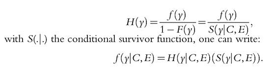
The trick is then to estimate a hazard-function-based estimator and introduce covariates using a proportional-hazards model. In a second step, the necessary transformations using the above equation are made to obtain an estimate of the associated conditional density function. It is known that the estimation of duration models is more flexible than of linear models. In substance, Pistolesi estimates the conditional distributions corresponding to Equations (4.16) and (4.17) with this estimation technique.

4.10.2.2 The Case of a Poor Data Set

The distinctive feature of a poor data set is that no effort variable is available, but we may still have a rich set of circumstances and a large sample. We can construct types but we cannot a priori build tranches. The approach here comes from Roemer (1993, 1996, 1998) with his identification axiom. It is the only assumption that enables us to say some­thing about inequality of opportunity in the poor-information case. It is nonparametric in essence, since effort is deduced from the distribution of outcome for a type, F(y ∣ C). Two individuals located at the same quantile of their type-conditional distribution are defined as having exerted the same effort, which will be denoted e_RO. Formally, starting from the income-generating process given by

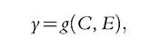
the Roemer identification axiom (RIA) reads:

By construction, this effort is distributed uniformly over [0, 1] for all types. This way of identifying effort has been used by O’Neill et al. (2000) in a nonparametric setting to depict the opportunity set of an heir defined as the income range that she can reach for all levels of Roemerian efforts belonging to [0, 1]. The opportunity sets are contrasted according to the level of advantage given by the decile of parental income.

This way of identifying effort has also been used by Peragine (2004) to build a tranche approach to EOp where the multivariate distribution is described by a matrix whose typical element is the income for a given type and percentile of the type-conditional income distribution. However, this approach is not immune to the omitted variable problem that was discussed above. As was rightly pointed out by Ramos and Van de gaer (2012), omitted circumstances induce wrong identification of the Roemerian effort unless the unobserved circumstances, after conditioning on observed circumstances, no longer affect income (see their Proposition 6). This is a strong condition that will be rarely be satisfied in empirical work.

The identification axiom may be questionable from an analytical point of view (see Fleurbaey, 1998), because it is not clear how multidimensional effort can be aggregated into one indicator, and luck factors can interact with effort in a complex way. The view that the distribution of effort specific to a type is a circumstance makes sense in the control view but not in the preference view. Let us coin this axiom as the type-independent effort distribution: the relevant normative effort distribution should be independent of type. This axiom is clearly weaker than Roemer’s identification axiom. It has inspired fruitful empirical strategies, both in a parametric and nonparametric setting. In the former case, Bjorklund et al. (2012) estimated a reduced form as in (4.18) with υ_i a Gaussian white noise. They assimilate the distribution of the residual to the distribution of effort. How­ever, the distribution of the residual can vary across types and this variation is a nonre­sponsibility characteristic. They have corrected for variation in the second moment by adding and subtracting to the regression equation a residual term that has the overall var­iance. Hence, the relevant effort in each type is renormalized to have the same variance.

In a nonparametric setting, Lefranc et al. (2009) retain this independence view of effort, which is postulated in the Roemer identification axiom, without assuming that we can identify effort with the quantile of the type-conditional income distribution. Let the distribution of effort conditional on type (supposed to be unidimensional) be given by G(e∣C). The authors follow Roemer’s proposition (see Section 4.3) according to which the accountable effort π is given by the quantile within the effort distribution of an individual’s type: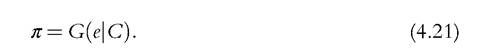

Equipped with this conception of effort, they are able to link what we can check (in a poor setting) with what we would want to check if we had all the information about effort. What we can check is obviously the equality of the distribution of income con­ditional on the observables, here, only the vector of circumstances: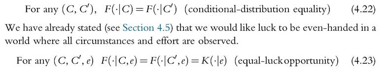

This allows the distribution of episodic luck to depend on effort but not on circum­stances. Their main result, mathematically obvious but of practical importance, is that a necessary condition for equal-luck opportunity to be satisfied is conditional­distribution equality, if we use relative effort. Mathematically, if we replace e by e_r, in (4.23), then (4.23) implies (4.22). Lefranc et al. (2009) prove that this is still the case if some circumstances are not observed. Checking the conditional-distribution equality on the set of observed circumstances is still necessary for the global EOp condition to be satisfied. These results pave the way for using stochastic-dominance tools³⁹ to measure the unfairness of the distribution, which we discuss below.

4.10.3 The Measurement Phase

Once a model has been estimated, the question of how to proceed to use the estimates obtained in the econometric phase remains open. Various choices have been proposed concerning three issues: the types versus tranches approach, the direct unfairness (DU) versus the fairness gap (FG), and the inequality index. We will deal with these three approaches in turn.

4.10.3.1 TypesVersusTranches

A way to organize the information in a discrete setting is to construct a matrix in which rows are types and columns effort. An element m_ij of the matrix is the outcome for type i and effort level j: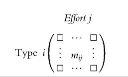

It is important to emphasize that this way of proceeding is correct if and only if the knowledge of circumstances and effort is sufficient to determine the outcome level. It means that, with respect to the decomposition of the process allowed by the regression, the residual is assigned to either effort or circumstances, unless the outcome is replaced by the predicted outcome. In this setting, two principles of compensation can be stated. First, we define a tranche as the set of individuals who expend the same degree of effort.

The tranche-compensation principle states that the closer each column is to a constant vec­tor, the better. If for some effort (column), the inequality of outcome across types is reduced, and everything else remains unchanged, EOp has been improved.

The type-compensation principle states that it is good to transfer from an advantaged type to a disadvantaged type, provided that the ranking of types is respected. Suppose that

39

It is possible to go beyond stochastic dominance to define the relative advantage of a type (see Herrero et al., 2012, for a proposal involving an eigenvalue of a matrix).

between two types, one is unambiguously better off than the other, that is, the outcomes can be ranked unambiguously according to first-order stochastic dominance. Then a transfer from the dominant type to the dominated type for some effort level, ceteris par­ibus, is EOp enhancing. This principle can be extended further to a second-order stochastic-dominance test (Lefranc et al., 2009). Indeed if two types have the same aver­age outcome but the first one has a larger variance, any risk-averse decision maker would prefer to belong to the second type and consequently one cannot declare that the two types have the same opportunities in terms of risk prospects. The need to take into account the risk dimension echoes the treatment of heteroscedasticity of the residuals in the parametric case by Bjorklund et al. (2012). This extension leads to a weak criterion of EOp, which corresponds to a situation of absence of second-order stochastic domi- 40

nance across types.

Fleurbaey and Peragine (2013) show by the means of an example that the two prin­ciples clash. There is no complete ordering of the full domain of (positive) matrices, which respects both principles. If we connect this to the results obtained by Lefranc et al. (2009), it is as if we said that equal-luck opportunity conflicts with conditional-distribution equality. ¹ They claim that a choice should be made between the two principles. Logically this is correct. Empirically, it seems to us, that the conflict is not that deep because the principles are useful in different informational contexts. Either one trusts the information about effort and the tranche-compensation principle is appropriate, or one lacks the information about effort, or believes it is insufficiently reliable because of the omitted-variable problem, and then the type-compensation principle remains available.

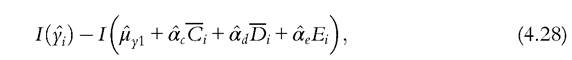
Fleurbaey and Peragine (2013) also point out that the tranche-compensation principle clashes with two principles of reward, the principle of natural reward and the principle of utilitarian reward. Ramos and Van de gaer (2012) showed that this incompatibility extends to another principle of reward inspired by a criticism of Roemer against the prin­ciple of natural reward. The principle of inequality adverse reward requires that a within-type Pigou-Dalton transfer be socially desirable.^{[161] [162] [163] It seems to us that this kind of conflict should not be overemphasized if we agree to prioritize the principles. Ifwe annihilate the inequality due to circumstances according to the tranche-compensation principle, then in each column, each element is equal to its tranche average before the redistribution took place. Hence, this redistribution according to the tranche-compensation principle respects a simple natural arithmetic average reward principle: The arithmetic average income difference due to differences in effort should remain invariant to redistribution. At this stage, this principle of reward reduces to the principle of natural reward and no more redistribution is required to comply with the requirements of EOp.}

We conclude with an insight borrowed from Ramos and Van de gaer (2012), who remark that if we retain the Roemerian effort, annihilating inequality within the columns of the matrix implies equalizing the prospects for each type, since by construction the distribution of Roemerian effort is the same for every type.

4.10.3.2 DU Versus FG

Almost the same idea appears in the papers of Fleurbaey and Schokkaert (2009) and Pistolesi (2009) concerning how to measure inequality due to circumstances. We will here retain the nomenclature of the former authors, while we are closer to the latter in terms of the definitions. These authors propose two approaches.

DU is computed as the inequality of the counterfactual distribution when one has removed the effect of effort variables, either by suppressing them, or by imputing to each individual a reference value of effort such as the average value. Following are some exam­ples of possible computations of DU, where I denotes some inequality index.

For the reduced form (4.18), a natural choice for DU is to compute the inequality of the conditional expectation of outcomes across types (a solution first proposed by Van de gaer, 1993). Since the regression decomposes the conditional expectation, we get which is a neat solution chosen by Ferreira and Gignoux (2011). The residual is set to 0, its mean value.

For the more structural model (4.16) or (4.19), where an estimation of the impact of the effort variable has been obtained, it is possible to set the effort variable to 0 or to con­sider some reference value such as the average effort. The inequality of the conditional expectation of outcome for an average effort level is given by where an overbar on a variable denotes a mean. A potential problem for both the above calculations is that the distribution of estimated residuals across types may be type depen­dent. If so, then the difference in the mean of estimated residuals across types should be taken into account.

The FG measures the gap between the inequality of the actual distribution and the inequality of a counterfactual distribution in which all the effects of circumstantial vari­ables have been removed, either by suppressing them, or by imputing to each individual a reference value of circumstances such as the average one. We give some examples below. If we had estimated a reduced form with only effort variables (something that has not been done in the literature so far), we could have the analog of formula (4.24) with an estimation of the inequality of the expected outcomes across tranches when circum­stances are in the residual and have been removed. Computing directly from the data the average outcome of those sharing the same effort, as done by Checchi and Peragine (2010), is a nonparametric way of doing this. The FG is then given by^[164]

Forthe more structural model (4.16) or (4.19), where both effort and circumstances vari­ables are introduced as regressors, we can do better and estimate the FG for a counter- factual distribution where the set of circumstances has been set to a reference value, for example, the average one. Then, one obtains for the FG

Bourguignon et al. (2007) propose a similar measure. The problem is, again, how to assign the residual. According to (4.27), the residual has been removed and is considered as measuring a circumstance. The above authors implicitly consider the residual as mea­suring effort. Another solution is to replace the overall inequality by the explained inequality, that is, remembering that y_i is the explained outcome (see Equation (4.20)), to compute:

a solution chosen by Jusot et al. (2013).

The reference values in (4.26) and (4.27) are somewhat arbitrary and we can compute the formula for different values and then take the arithmetic mean. DU and FG as defined above are defined in absolute value. They can of course be defined in relative terms and be divided by the overall inequality. Several recent empirical studies (e.g., Aaberge et al., 2011; Checchi and Peragine, 2010) perform both estimations of the inequality of oppor­tunity as robustness checks.

The measurement of unjust inequality using DU is linked to the tranche-compensation principle as follows: if DU computed according to formula (4.25)^[165] for some matrix M is lower than for some other matrix M for all inequality indices, then M is preferred to M according to the tranche-compensation principle where the considered transfers are of the Pigou-Dalton sort. Similarly, there is a link between the type-compensation principle and the FG. Indeed, if Mis preferred to M according to the type-compensation principle,

then the FG is lower for M than for M, computed according to (4.27), for all inequality indices when the reference type is different from the two types involved in the Pigou- Dalton transfer. The statement is not as general for FG as for DU since we cannot extend the above statement whatever the reference type, the choice of which is ad hoc. This leads some authors to consider instead a weighted average of the FG. In that case it can be proved that, if M is preferred to M according to the type-compensation principle, then the weighted^[166] sum of the FGs is lower for M than for M, computed according to (4.27), for all inequality indices belonging to the entropy class.^[167]

We conclude the discussion ofDU and the FG by observing that the concepts in sub­stance are not new as methods of decomposing inequality among its sources. When Shorrocks (1980) advocated the use of the variance, he observed in his conclusion that when one thinks about the contribution of one source to inequality, one can wonder either about how much inequality is left when the impact of this inequality factor is neu­tralized, or about how much inequality remains when the other sources are equalized. This is exactly the choice available in the literature on EOp measurement. Shorrocks (1980) also observed that when there are two sources (here, the set of circumstances and the set of effort variables) the natural decomposition of the variance given by the covariance of the source with outcome has a nice interpretation: the covariance of a source is just equal to the arithmetic mean of the above two computations. In the context of EOp, this means that the covariance of circumstances with outcome is the arithmetic mean of the DU and FG when the other source is removed in the computations (not put at a reference level). This point was made by Jusot et al. (2013) and by Ferreira and Gignoux (2011) (see their appendix).

4.10.3.3 TheChoiceofanIndex

The entire spectrum of inequality indices has been used by researchers in EOp, perhaps with the exception of Atkinson’s indices. One can speculate that the absence of the Atkinson indices is due to EOp’s not being a welfarist theory. Lefranc et al. (2008) and Almas et al. (2011) have used the Gini index, and Aaberge et al. (2011) have used the Gini and other rank-dependent measures. Elements of the entropy family have been used by Bourguignon et al. (2007), who picked the Theil index, and Checchi and Peragine (2010), Ferreira and Gignoux (2011), Lefranc et al. (2007, 2012) use the MLD. Pistolesi (2009) and Bjorklund et al. (2012) are eclectic and use a range of mea­sures. These examples are when the objective is income attainment, and they are relative measures. When the objective is health status (self-assessed health or mortality), it makes sense to use an absolute measure such as the variance, a choice made by Jusot et al. (2013) and Bricard et al. (2013), which possesses the decomposition property mentioned above. However, the variance is not such a good choice for income attainment since it is not relative. Returning to the income case, there is no first-best choice. The connection with stochastic dominance, which is the advantage of rank-dependent measures (among them the Gini index), is counterbalanced by the decomposability properties of the entropy family. The relevant decomposition is among sources of inequality, and not so much among subpopulations, and the Shapley decomposition (Chantreuil and Trannoy, 2013; Shorrocks, 2013) can be applied to any inequality index.

The property of path independence of the MLD pointed out by Foster and Shneyerov (2000) has recently been emphasized by Ferreira and Gignoux (2011) to single out this index. Indeed, path independence is interesting in the context of EOp because it can be interpreted as saying that the inequality measured by the DU criterion be equal to the inequality measured by the FG. This proposition has to be qualified. DU is computed as the inequality of the average outcome across types. The FG is obtained by rescaling the distribution of the outcome due to effort by the ratio of average income to average income in a type. This is one among many possibilities for nullifying the impact of cir­cumstantial factors. Thus, if we find this way of neutralizing the impact of circumstantial inequalities appealing for the FG, then we do not have to worry about computing two measures of EOp because they are equivalent (under path independence). We conclude by saying that in the health realm, variance may be a better choice, whereas MLD is prominent for income achievement.

4.11.