Intragenerational mobility: evidence
This section assesses evidence about within-generational income mobility. It first considers definitional issues, the nature of the longitudinal data available, and issues of empirical implementation, and then it turns to the evidence itself.
Our review of the topics is selective. We draw on and refer readers to Jenkins (2011a, chapters 2 and 3) for a much more extensive discussion of data sources for within-generation mobility and related empirical issues, as well as extensive references to other literature. Our survey of evidence concentrates on findings emerging over the last two decades, and gives greatest attentionto the United States, with examination of trends over time and cross-national comparisons between the United States and (Western) Germany, but studies for other countries are also considered. Our focus reflects the emphasis in research to date, and this, in turn, is related to the availability of suitable data (as we explain). Also, to make the review manageable, the focus is on mobility of household income rather than of individual labor earnings (though selected earnings studies are referred to). We show how conclusions about trends over time and cross-national differences vary with the mobility concept chosen.
Issues of statistical inference are ignored here. On these, see, e.g., Biewen (2002) and Chapter 7.
10.4.1 Data and Issues of Empirical Implementation
Any study of income mobility faces three “W” issues: mobility of What, among Whom, and When? Studies of trends over time or across countries add another issue, that of comparability. The choices that researchers can make under these headings are much constrained by the sources of longitudinal data that are available. But the data situation has improved substantially over the last two decades. (Contrast the situation described later with the discussion by Atkinson et al., 1992, chapter 3, which focuses on earnings.) Although many of the “W” issues arise in any study of income distribution, looking at mobility adds some extras twists to those arising in cross-sectional analysis.
Mobility of “What” refers to which income sources are included in the definition of “income.” Definitions typically range from measures with only a single source (typically earnings from employment) to a broader measure such as household income, which includes multiple sources. Many variations are possible (e.g., labor earnings may refer to employment earnings only, or earnings from all jobs that an individual has, and may also include self-employment earnings, thought often not). There are multiple definitions of income as well. The most common distinction in empirical work is between measures of pretax pretransfer income, pretax posttransfer income, and posttax posttransfer (also often labeled original or market or pregovernment income; gross income; and net, disposable, or postgovernment income, respectively). Pregovernment income typically includes labor earnings, income from savings and investments, and transfers received from nongovernment sources. Taxes usually refer to taxes on income (typically at national level, sometimes also including local taxes) and contributions levied for public pensions. “Transfers” usually refer to cash benefits received from the state.
Mobility among “Whom” refers to the definition of the income-receiving unit. Clearly this is closely related to the issue of What. For example, it is individuals that receive labor earnings. Benefits are assessed and income taxes levied on families and
33
For a comprehensive discussion of the various definitions and recommendations for measurement, see Expert Group on Household Income Statistics (The Canberra Group, 2001). households. Individuals not in paid work such as stay-at-home mothers or children, often do not receive income in their own right, but benefit from income sharing with families and households. Putting things another way, note that analysis of earnings mobility is typically restricted to workers with earnings, excluding those without earnings, many of whom are women, children, or of retirement age.
In contrast, it is typically assumed that each individual receives the (equivalized) total income of family (or household) to which he or she belongs. Because total household income is rarely zero, all individuals, regardless of age or labor market attachment, can in principle be included an analysis of income mobility. There is no universally correct definition of the income unit, and which should be used depends on the goals of the mobility analyst. For example, in a study of labor market flexibility, a focus on individual earnings is appropriate (though there remain questions about whether women can and should be included in such analysis—much empirical analysis is of men only). On the other hand, if the interest in mobility is stimulated by a desire to describe and summarize important features of society as a whole, then there is a strong case for using more inclusive samples. As we show later, some empirical studies focus on individuals of working age (variously defined), others on all individuals, and this can complicate cross-study comparisons.“When” mobility issues refer to two aspects related to time. The first is the length of the period to which income refers to. For instance, is it the hour, week, month, or year? Economists often argue in favor of longer reference periods (e.g., a year) on the assumption that temporary variations and measurement error are smoothed out, thereby providing a more accurate measure of living standards. There is relatively little empirical evidence available about the veracity of this hypothesis because analysts rarely have income data for the same people over both shorter and longer periods. Boheim and Jenkins (2006) surveyed the literature and, from their analysis, argued that income mobility calculated using current (monthly) and annual income definitions are similar, and they provide a number of data-related reasons. Canto et al.’s (2006) analysis is more comprehensive; based on comparisons from quarterly and annual income data for Spain, they show that use of the longer assessment period leads to higher estimates of poverty prevalence, lower inequality, and less mobility.
A second “When” issue relates specifically to mobility analysis in particular rather than income distribution analysis in general. For much mobility analysis, the data refer to a bivariate income distribution in which the marginal distributions refer to 2 years, t and t + #964;, and empirical analysis of longer-term inequality reduction requires a definition of how many years constitutes the longer term. In both cases, how far apart the base and final years are will affect the conclusions because the longer the interval, the greater the possibilities of mobility (as we illustrate later).[603] Choices about what interval to use have implications for the analysis that one can undertake too because data sets cover a time period Ofparticularlength (rarely more than 20 or 30 years), so researchers can only look at mobility trends if they use relatively short time windows for their measures. The constraint becomes acute with longitudinal data sets like EU-SILC (discussed later) in which the maximum time period is 4 years.
34
How researchers can address the three “W” issues is much constrained by the data that they have available to them, and this raises issues of comparability over time and country. Longitudinal data sources suitable for within-generation income mobility analysis are of two main types.
First, there are household panel surveys in which nationally representative samples of the private household population are interviewed about their incomes and many other domains of their lives in an initial year and then reinterviewed thereafter at regular intervals (usually a year). Second, there are administrative registers (e.g., tax files) in which income records for individuals are linked longitudinally. Household panel surveys typically utilize income definitions (i.e., resolve the “What” and to “Whom” issues) that are consistent with definitions accepted as being of good quality in large cross-sectional surveys. By contrast, administrative record data are typically designed for administration of the tax and benefit system, and the definitions used of income and the income-receiving unit, and the population that is represented, are determined by the needs of administration rather than by research.
But register data also have advantages relative to surveys: Their samples are very much larger, issues of respondent dropout or measurement error do not arise in the same way (see the discussion later), and coverage of the very richest income groups is much better (they are typically not reached by surveys).The clinching argument for empirical researchers in favor of household panel surveys over administrative registers is that the former became widely available for many countries, especially from the mid-1980s onward, with cross-nationally harmonized versions of the data following a few years later. Administrative registers with longitudinal income data have remained rare until recently in most countries, with the exception of Scandinavian countries, which have a rather longer history of use.
The longest-running household panel is the U.S. Panel Study of Income Dynamics (PSID), which began in 1968 and still continues, though it changed from annual interviewing to biennial interviewing after 1997. Panels started in the early 1980s in the Netherlands and Sweden, but the most well-known European panel is the German Socio-Economic Panel (SOEP), which started in the 1984 and is still running. Other country panels include the British Household Panel Survey (BHPS), which started in 1991 and finished in 2008. (The BHPS was recently replaced, after a break, by a new and very much larger panel (Understanding Society), which incorporates most of the original BHPS sample.) The Household, Income and Labour Dynamics in Australia (HILDA) survey began in 2001 and is ongoing. There is also Survey of Labour and Income Dynamics (SLID) for Canada, which is a rotating panel operational between 1998 and 2011.
As shall be seen later, it is the household panels cited in the last paragraph that have provided most of the empirical evidence about income mobility over the last two to three decades, both in their native format (often to examine trends over time within a country) or in a harmonized form (to undertake cross-national comparisons).
The production of cross-nationally comparable household panel data with harmonized labor earnings and household income variables has been one of the major successes in social research infrastructure creation over the last few decades.The Cross-National Equivalent File (CNEF) began in 1991 with harmonization of data from the U.S. PSID and German SOEP and incorporated the BHPS and SLID in 1999 and HILDA in 2007. (Data for more countries have been added subsequently.) It should be stressed that the project does more than simply harmonize variables; it adds value. One important example of this is the derivation of comparable posttax posttransfer household income variables. The original PSID family income variable refers only to pretax posttransfer income, and the government transfers do not include income derived from nonrefundable tax credits (the EITC) or near-cash benefit income in the form of Food Stamps (now called SNAP). The CNEF uses the NBER TAXSIM model to simulate taxes. Similarly, involvement in the CNEF project was a stimulus for the SOEP to develop and maintain a similar model in-house. (Other CNEF members also use such models.) For a more detailed discussion of the CNEF, see Frick et al. (2007).35
Another important initiative providing cross-nationally comparable panel data on incomes was the former European Community Household Panel (ECHP), though this has been used less often for mobility analysis than the CNEF and its constituent panels. The ECHP relied on “input” harmonization by contrast to the CNEF’s “output” harmonization. That is, household panel surveys with the same design and questionnaires including the same variables were fielded in a number of countries, so that harmonization was built in from the start. Data from a maximum of eight annual interview rounds are available, covering the period 1994—2001. Twelve EU member states participated in the ECHP initially, with two more joining shortly thereafter. The ECHP never realized its full potential because, for many years, researcher access to the data was constrained and financially costly. This is in contrast with the CNEF, which from the start has had a much more open data access policy and has been more research(er) driven.[604] [605] The ECHP was replaced—after a gap—by the European Statistics on Income and Living Conditions (EU-SILC) from 2005. EU-SILC is explicitly designed to deliver data on a set of social indicators that include income distribution statistics. This is output harmonization again, though the target variables are predefined by the needs of EU policy making rather than by researchers. Some member states use administrative registers to produce the data; others use panel surveys, an aspect that has led to questions about data comparability (see later). The longitudinal data in the publicly released EU-SILC data sets track individuals for a maximum of 4 years (by design), and so the scope for longer-run mobility analysis is ruled out. The great advantage of the EU-SILC longitudinal data is that, when mature, they will cover all EU member states. Understandably the EU-SILC has not been much used for income mobility to date, and this is reflected in our review of evidence that follows. This review of data sources suggests that there has been a substantial increase over the last three decades in the volume of high-quality longitudinal data available to researchers. But there remain a number of important issues of empirical implementation that need to be kept in mind when assessing the value of a particular mobility study. So, before turning to discuss empirical evidence, we briefly review these issues. There are generic issues associated with longitudinal surveys, notably the potential problem of survey attrition. Over time, some respondents to a panel survey drop out from the data, either no longer wishing to participate or unable to be tracked down for interviews. Attrition has two potentially adverse effects. The first is reduction of sample size, with consequences for the precision of estimates. The second potential effect, more commonly discussed, is on the representativeness of the sample. Particular groups such as young people tend to be more likely to drop out, in which case estimates may be biased.[606] Differential attrition may be related to both observed and unobserved characteristics of individuals and families. For the former case, data producers routinely produce and release sets of weights that can be used to maintain the representativeness of estimates, and virtually all the studies cited in our evidence review use these weights. By definition, it is harder to assess the effects on estimates of differential dropout related to unobserved characteristics; it requires modeling of the attrition process. For an extensive discussion of attrition in U.S. household panel surveys, see Fitzgerald et al. (1998) and other papers in the Summer 1998 issue of the Journal of Human Resources. The likely impact of attrition is associated with the type of mobility analysis undertaken. Attrition between successive waves of a household panel is typically relatively low (around 5%) with the exception that dropout rates are noticeably greater between the initial and second waves. Estimates of mobility over short periods (1 or 2 years, say) are likely to be less affected by attrition than estimates based on long runs of data. Respondents may remain in a longitudinal survey, but not provide complete responses to particular questions, either because they do not understand the question, do not know, or do not wish to provide the answer. This is the issue of “item” nonresponse leading to missing data for some respondents and, as with attrition, may be associated with both observed and unobserved respondent characteristics. Item nonresponse is particularly prevalent for questions about income sources by comparison with items such as, e.g., a respondent’s age. In the public-use panel data sets used by mobility researchers, missing income values are typically replaced by an imputed value (together with a flag that enables identification of such observations) generated using procedures allocating similar values to respondents with similar sets of (observed) characteristics. Imputation is very useful for analysts but can potentially have effects on analysis because, by comparison with nonimputed data, extra “noise” is added by the inevitable imperfection of the process.[607] These can have particular effects on mobility analysis because some of the changes in a person’s income over time may simply reflect the imputation process in the different years. But if one simply drops the imputed observations, there may be a critical loss of sample size and use of a potentially nonrepresentative subsample. In most of the income mobility studies discussed later, analysts have routinely used imputed data on household income. By contrast, in studies of earnings volatility, it is a more common practice to drop imputed observations. Researchers tend to find that this reduces observed volatility, but the effects are relatively small. Again, the likely effects will depend on whether the particular mobility measure employed requires, say, two years relatively close together, or many years over a longer interval. The problems raised by imputation are closely related to the more general issue of measurement error in earnings and income data. Even if survey participants respond to a question, their answer may be incorrect either because the respondent does not want to give the true answer or simply does not know what it is. Key issues are whether observed responses are systematically under- or overreports of the (unobserved) true value or simply random, and how errors are correlated across successive years of data for the same respondent. Clearly, the answers to these questions may differ by income source. The largest body of research on measurement error has been about labor earnings and used validation studies in which linked administrative record data are used to provide a picture of each worker’s “true” earnings (see, e.g., the survey by Bound et al., 2001). Few studies have looked at the effects of measurement error on measures of earnings mobility. The perhaps surprising finding of Gottschalk and Huynh (2010) is that estimates of men’s earnings mobility, defined in terms of the Pearson correlation between log earnings in 1 year and the next, are much the same in the survey data and their administrative data set. The result arises not because measurement errors are not important; rather, it is because they are “nonclassical” in nature (i.e., mean-reverting and correlated across years), and these various features happen to offset each other. See also Fields et al. (2003), who use a nonclassical measurement error model similar to that of Gottschalk and Huynh (2010) to put bounds on estimates ofincome change. For the case considered, they argued that the effects of measurement error are “relatively minor” (Fields et al., 2003). Dragoset and Fields (2006) calculated a large portfolio of mobility measures from both survey and linked administrative record data on U.S. men’s earnings. They concluded that most of their qualitative results are the same in both data sources, and that the estimates from the administrative source were neither systematically above nor below the corresponding survey estimates. Overall, this small body of research might be taken to imply that measurement error has relatively unimportant effects on measures of mobility in practice. We would caution against this interpretation, convenient as it is for empirical researchers; the situation is more that we know rather little at present. All the studies cited refer to earnings for U.S. men, and results may differ for household income and in other countries. (The only similar study for household income that we are aware of is by Rendtel et al, 2004, who also reported finding mean reversion and serial correlation.) There is also a more fundamental question of whether administrative record data can be assumed to provide error-free representations of the truth (Abowd and Stinson, 2013).[608] 38 A rather different sort of measurement error arises in the case of outlier observations, for example, very high or very low observations. These may be genuine but may also represent errors of, e.g., transcription leading to additional zeros being added. The problem is that even if the number of observations with this kind of data is very small, they may have a big influence on the estimates that are derived. This lack of robustness is undesirable. See Cowell and Schluter (1999) for a discussion of this problem in the context of income mobility analysis. Empirical analysts’ response to this issue is usually to simply drop a fraction (e.g., 1%) of the very richest and of the very poorest income values in each year. This procedure, known as “trimming,” or similar algorithms directed at removing potential outliers, has been applied in virtually every study cited in our discussion of empirical evidence. A final empirical issue is whether income changes over time represent genuine mobility or, instead, systematic changes associated with life cycle patterns of such earnings following an inverse-U shape with age. Many income mobility studies do not adjust for this factor; they look at observed incomes. Some other studies, mostly of earnings mobility, have regressed observed earnings against variables such as age, and then the mobility analysis is of the earnings residuals: see later discussion. 10.4.2 Intragenerational Income Mobility in the United States: Levels and Trends We take as our initial reference point the estimates of income mobility for the United States provided by Hungerford (2011), as he uses good-quality comparable data from PSID (as released via the CNEF) and provides a range of mobility summaries. (Transition matrices from the study were presented in Table 10.1 earlier.) Hungerford compared mobility over two 10-year intervals, 1979-1988 (“1980s”) and 1989-1998 (“1990s”). The measure of income is annual disposable (posttax posttransfer) family income adjusted for differences across families in household size and composition using the equivalence scale proposed by Citro and Michael (1995). His samples include all individuals within households. In the 1980s sample, about half the SEO sample was dropped in 1997. All estimates are derived using the PSID’s weights. We noted earlier that, in both periods, there appeared to be substantial short-distance mobility over a 10-year period, but long-distance moves were relatively rare. Moreover, the chances of upward mobility from the bottom and downward mobility from the top appeared symmetric. We now compare mobility in the two decades in greater detail, in particular considering whether mobility increased or decreased according to various mobility concepts and measures. To assess changes in positional mobility, a natural first approach is to apply the dominance check of Atkinson and Bourguignon (1982) based on the differences in the discrete cumulative densities implied by the decile transition matrices in Table 10.1. See Table 10.2 for the estimated differences. First-order dominance does not hold; there is a mixture of positive and negative differences.[609] There is an interesting pattern, however. Most of the positive differences (greater cumulative density in the 1980s) are found in cells corresponding to movements out of or into the poorest fifth of the distribution. Put another way, there is greater movement in the 1980s than the 1990s into and out of the richest 80%, broadly speaking. Saying conclusively that mobility increased or decreased in the United States between the 1980s and 1990s, and by how much, requires additional assumptions about the weighting of mobility in different parts of the distribution. Also, the answers depend on the mobility concept. These points are illustrated by the mobility index estimates reported by Hungerford (2011) and summarized in Table 10.3. The first three rows Table 10.2 Differences in cumulative density: United States, 1979-1988 versus 1989-1998 Note: The estimates are in percent, rounded to one decimal place, and show in each cell the cumulative discrete density for the 1980s minus the corresponding cumulative discrete density for the 1990s. Source: Authors' calculations from Hungerford (2011, Tables 2 and 3), based on PSID data. Table 10.3 Selected mobility indices (%): United States, 1979-1988 versus 1989-1998 Index 1979-1988 1989-1998 Note: The estimates are in percent, rounded to one decimal place, apart from those in the last two rows (in constant-price dollars). Decile mobility is the proportion of persons changing at least one decile group. The normalized trace is the Shorrocks (1978b) index calculated from the decile transition matrix. The Gini mobility index is the index of Yitzhaki and Wodon (2005). The Equalization indices are those of Shorrocks (1978a) and Fields (2010). On the average ofabsolute income and income share changes, see Fields and Ok (1996) and Fields (2010). See text for more details. Source: Authors' calculations from Hungerford (2011, Tables 4 and 8, and p. 97), based on PSID data. of the table provide estimates ofpositional mobility (reranking), and all the indices show a small decline between the 1980s and 1990s. In contrast, the Shorrocks and Fields equalization indices record an increase, and so too do the two measures of income flux shown in the bottom two rows. For the last four indices, the estimated increase is small, with the exception of the Fields equalization measure, for which the large change reflects the increase in (cross-sectional) income inequality over the period. The general lesson is that conclusions about whether mobility increased or decreased between the 1980s and 1990s depend on the mobility index employed. Figure 10.9 Median real income growth, by base-year decile group: United States, by period. Note: The estimates show median income growth for each base-year decile group over the relevant period. Source: Hungerford (1993, Table 9) and Hungerford (2011, Tables 5 and 6). Mobility as individual income growth is also summarized by Figure 10.9, which shows the median real income growth for each base-year decile group, by period. (This is a grouped data version of Figure 10.7 discussed in the previous section.) Clearly income growth is pro-poor in the United States (consistent with regression to the mean), but the patterns differ between the 1980s and 1990s. Income growth was greater in the 1990s than the 1980s for the richest eight base-year decile groups, but no different for the two poorest base-year decile groups. The extent to which U.S. mobility comparisons can be extended to periods before the 1980s and after the 1990s is restricted by data availability (e.g., the PSID only started in 1968) because different studies use different income variables and estimation samples and often do not report the same mobility statistics. For example, Hungerford (1993) provides much information about U.S. income mobility in the 1970s and 1980s, but the estimates are not fully comparable with those in Hungerford (2011) because the earlier study uses a different income definition (pretax posttransfer income rather than equivalized posttax posttransfer income), and the interval between base- and final-years differs (8 years rather than 10; e.g., 1979-1986 rather than 1979-1988). The relevance of definitional differences is illustrated by the estimates for the “1980s” from the two studies of the proportions ofindividuals remaining in the poorest 10th and remaining in the richest 10th: 44.3% and 40.0% according to Hungerford (2011), but 49.0% and 42.1% according to Hungerford (1993, Tables 1 and 2). Look also at the different estimates of real income growth rates for the 1980s for the two periods in Figure 10.9. Using the Hungerford (1993) definitions, the overall growth rate for the 1980s is smaller (which is unsurprising because aggregate income growth was positive throughout the mid-1980s; Hungerford, 2011, Table 1), but observe that the estimates of pro-poorness in income growth also differ (the income growth curves from the two studies do not have the same slope). One can compare mobility in the 1970s and the 1980s, however. Ifwe examine differences in cumulative densities using Hungerford’s (1993) estimates, again there is no clear-cut mobility ordering (authors’ calculations), and there is a broadly similar pattern of differences to that described earlier. Hungerford (1993) does not report summary indices to compare with those in Table 3, but two statistics based on the transition matrices (Cramer’s V) and the contingency coefficient “are the same... suggesting that the degree of association between a person’s decile rank in one year and another was the same in the 1970s and 1980s” (Hungerford, 1993, p. 407). Fields and Ok (1999a) used exactly the same data as Hungerford (1993) and reported that their measure ofincome flux, the average of the absolute changes in log income, increased from 0.498 in the 1970s to 0.528 in the 1980s.[610] So, again, changing the mobility concept leads to a different conclusion about trends. Hungerford’s (1993) study is also useful because it analyzes whether the estimated mobility patterns are robust to adjustment for transitory income variation. Specifically, Hungerford calculated each individual’s 5-year longitudinally averaged income (centered on the year in question) and used these “permanent” incomes instead of the single-year incomes to define base-year and final-year income positions. Interestingly, the patterns of mobility revealed are remarkably similar, though with perhaps less movement at the top and bottom of the distribution.[611] For example, according the annual income calculations for 1979—1986, 12.9% of the poorest fifth remain in that group and 11.0% of the richest fifth remain in that group. According to the permanent income calculations, the corresponding estimates are 11.5% and 9.6% (authors’ calculations from Hungerford, 1993, Tables 2 and 4). To examine trends in U.S. income mobility further, we turn to Bradbury (2011). She provides estimates using consistent definitions for the period 1969-2006 and for a large portfolio of mobility indices. Her estimates are not fully comparable with Hungerford’s, however. Although she and Hungerford (2011) both use posttax posttransfer real family income measures from the CNEF version of the PSID, they use different samples. Bradbury focuses on adults who are a family head or spouse rather than all individuals within families, both head and spouse (if present) are required to be of working age (16-62 years), and the time interval spans 11 years rather than 10. She used the square- root-of-household-size equivalence scale rather than the Citro and Michael (1995) one. Trends in three general indices of positional mobility are displayed in Figure 10.10: the fraction of individuals changing decile group (“decile mobility”), one minus Spearman’s rank correlation, and Yitzhaki and Wodon’s (2005) Gini mobility index. All three indices are broadly constant over the 1970s and decline over the 1980s (11-year intervals starting at the end of the 1970s), with the rate of decline perhaps slowing from the late 1980s onward. The fall in mobility over the 1980s is consistent with Hungerford’s estimates of trends based on only two intervals during this period, but is rather larger in magnitude. The Gini mobility index fell by about a sixth between the intervals starting in 1979 and 1989 (but only about 5% according to Hungerford, 2011). One minus the rank correlation fell by about one-fifth over the same period, and so the decline in positional mobility is relatively large. It is unclear what lies behind the secular decline in mobility, but we note that it was at the end of the 1970s that U.S. family income inequality also began to increase (Burkhauser et al., 2011), suggesting that inequality and positional mobility share some common drivers. There is no very obvious association between series’ turning points and the business cycle (there were recessions at the beginning of the 1970s and 1980s). Figure 10.10 Indices of positional income mobility: United States, 1970-1995. Note: The estimates refer to 11-year intervals, with incomes in base- and final-year averaged over 2 years. For example, the estimates labeled as 1970 refer to incomes longitudinally averaged over 1969 and 1970 (base year) and 1979 and 1980 (final year). See text for index definitions. Source: Bradbury (2011, Tables 2 and 3). The conclusions about trends cited so far refer to income changes over an interval of 10 or 11 years, and it is of interest to know how results change if rather different interval lengths are used. The research of Gittleman and Joyce (1999) suggests some sensitivity. Using PSID data for 1967—1991 and, like Bradbury (2011), focusing on working-age adults and employing a broadly similar income definition,[612] they calculated IRs, defined as the percentage of individuals remaining in the same fifth, for intervals of 1, 5, and 10 years. Gittleman andJoyce (1999, Table 1, Figure 2) show that the level of positional mobility increases (the IR falls) as the interval width is widened. But conclusions about mobility trends are also affected. For the 10-year interval case, there is a small downward trend during the 1980s consistent with Bradbury’s (2011) estimates. However, 5-year IRs exhibit no similar trend, and 1-year IRs generally decline from the end of the 1960s until the end of the 1970s and increase in the following decade (though the changes are not large in absolute magnitude). To provide a comparison with another commonly used mobility index, we also show trends in one minus Beta. It follows a different trend, which is perhaps unsurprising given that it is not a purely positional measure (see Section 10.3). Compared to the trends shown by the three positional indices, the decline during the 1970s is earlier and sharper, and there is no decline during the 1980s. The final two measures shown in Figure 10.10 are two “corner probabilities” from a quintile transition matrix (cf.Section 10.3), specifically the proportion of individuals in the poorest fifth in the base-year who are in a different fifth in the final year and, analogously, the proportion leaving the richest fifth over the relevant interval. These statistics pick up on particular aspects of positional mobility. Interestingly, it appears that the trend in the percentage leaving the richest fifth tracks the trend in overall positional mobility better than does the trend in the proportion leaving the poorest fifth. The estimates also bear on our earlier comments that the U.S. decile transition matrices for the 1980s and 1990s suggest that there is a broad symmetry to upward and downward mobility. We now see that asymmetry is more apparent if mobility is summarized using quintile rather than decile groups. In particular, it appears from Bradbury’s (2011) estimates that the chances of downward movement from the top (richest fifth) are typically several percentage points greater than the chances of upward mobility from the bottom. This asymmetry finding also may be contingent on the particular samples and other definitions used. For example, Bradbury and Katz (2002, Annex A) report quintile transition matrices for 1969—1979,1979—1989, and 1988—1998 using similar PSID samples to Bradbury (2011), except that “working age” now refers to a wider age range (head and spouse [ifpresent] less than 66 years), and family income is pretax postgovernment family income, equivalized using the PSID scale. The two probabilities are approximately equal in each matrix (50% in the first two periods, 47% in the last one). In contrast, Gittleman and Joyce (1999, Table 5) report quintile transition matrices for 1967-1979 and 1979-1991 using a similar income definition (but equivalized using the U.S. poverty line), and “working age” refers to head and spouse between 25 and 65 years. According to this study, the chances of leaving the poorest fifth are distinctly smaller than the chances of leaving the richest fifth (around 50% compared to around 60%). 43 Trends in mobility defined as equalization of longer-term incomes are summarized by Figure 10.11 using Shorrocks’s (1978b) measure M = 1 — R. The long series (shown in black) are derived from Bradbury (2011); we discuss the series in gray shortly. Although mobility levels differ substantially depending on which inequality index is used—there is much greater mobility according to the Theil index compared to the Gini—the patterns of change over time are the same according to the two series. There was a decline in mobility between the early 1970s and the mid-1980s, followed by a rise over the following decade, with leveling off around the mid-1990s. Although the changes are small in absolute terms, they are relatively large in proportionate terms. For example, between the mid-1980s and mid-1990s, the Theil-based measure increased by some 15% and the Figure 10.11 Mobility as longer-term income inequality reduction: United States, 1970-1995. Note: The estimates refer to the Shorrocks equalization measure, M frac14; 1 — R, calculated using the Gini and Theil inequality indices. The Bradbury (2011) calculations are based on 11-year intervals with longer-term average incomes calculated using every second year's income to handle the PSID's change to alternate-year interviewing in the late-1990s. The Bayaz-Ozturk et al. (2014) calculations use 5-year intervals, with interval base-years 2 years apart. Sources: Bradbury (2011, Table 4) for the series shown in black and Bayaz-Ozturk et al. (2014, Table A1) for the series shown in gray. Both use PSID (CNEF) data. Gini-based measure by almost 13%. The results are consistent with Hungerford’s (2011) finding of only a small increase in a Gini-based measure between the 1980s and 1990s, but Figure 10.11 shows that this is partly a consequence of the timing of measurement; Hungerford’s two intervals lie on either side of the bottom of a U-shaped series. Also, the turning points in the these two series differ from those for the positional measures shown in Figure 10.10, suggesting that the different aspects of mobility have different underlying causes. In addition, mobility according to the Shorrocks measure is much the same (Gini-based index) or greater (Theil-based index) in the mid-1990s than in the early 1970s, whereas mobility is lower according to the positional mobility indices shown in Figure 10.10. The research of Bayaz-Ozturk et al. (2014) allows to consider what happened to mobility as equalization after the mid-1990s. Although they also use a Theil-based measure, similar income measures, and the same data source, their series are not directly comparable with all individuals in families in their analysis samples (not only working-age adults) and they use a 5-year rather than 11-year interval. As a consequence, mobility levels are estimated to be substantially lower in all years (compare the gray line for the United States with the black one). Reassuringly, however, the series show broadly similar trends (and turning points) over the period for which they overlap. Bayaz-Ozturk et al.’s (2014) estimates indicate that mobility changed little in the second half of the 1990s, with a suggestion that it fell again in the 2002-2006 period. All estimates of trends in household income mobility presented so far in this section are based on PSID data, and it is of interest to know whether the evidence from other data sources tells a similar story. The main reference point on this issue is Auten and Gee’s (2009) work based on income data from tax administration records covering the two decades between 1987 and 2005. The data and definitions used are not fully comparable with those in the PSID studies, but there are advantages from having much larger sample sizes and much better coverage of top incomes. The analysis focuses on tax filers and their spouses (if present), excluding taxpayers aged under 25 years. An individual’s income is the income of the his/her tax filing unit, divided by the square root of household size. Income is a measure of pretax income and includes all taxable income sources reported on tax returns supplemented with data about Social Security benefit income provided to the Internal Revenue Service. The first part of Auten and Gee’s (2009) article describes mobility between 1996 and 2005 in terms of positional mobility (transition proportions) and income growth (by base-year income group). The results are broadly consistent with the studies cited earlier in terms of pointing to substantial movement between quintile groups but with shortdistance moves the most prevalent, and real income growth is greater the poorer the base-year income group. The distinctive feature of the study is the information about mobility at the very top of the distribution with mobility statistics also provided for the very top income groups. The authors report that there is a large amount of turnover at the top and that “the incomes of many taxpayers at the highest levels are very volatile” (Auten and Gee, 2009, p. 311). For example, among the richest 0.01% in 1996, only 23% remained in the group in 2005. Although over 80% were still in the top 1%, 6% dropped out of the richest fifth (Auten and Gee, 2009, p. 311). The second part of Auten and Gee’s (2009) article assesses changes in mobility between 1987 and 1996 and 1996 and 2005 using the same measures, and the authors state with regard to positional mobility that “the basic finding... is that [it] is approximately the same in the last 10 years as it was in the previous decade” (Auten and Gee, 2009, p. 311). Also, although overall real income growth was around 23% in the first decade compared to 8% in the second, its pro-poor pattern was similar across most of the distribution. (Median real income increased by about 15% points for the top four quintile groups and by about 10% points for the poorest base-year fifth). Things were different at the very top, however. Real income growth was —32% for the top 1% in 1987, and —31% for top the 1% in 1987 (Auten and Gee, 2009, Table 10.7). Further information about persistence in the top 1% is provided by Auten et al. (2013) for tax filers aged 25—60. Their Table 10.3 shows survival rates in the top 1% (i.e., taking taxpayers in this group in some base year t, what proportion of them were in the top 1% in each and every subsequent year t + #964;, where #964; = 1, 2, 3, 4, 5). Base years run from 1991 to 2009. The 5-year survival rates range between 21% and 36% and the 1-year survival rates between 52% and 70%. The authors pointed out that lower persistence rates tend to occur in recessionary periods (1991,1999 through 2001, and 2007), and they suggest that income sources of particular relevance for the richest groups such as capital gains and net business income are relatively sensitive to the business cycle. The body of evidence on trends in measures of mobility as family income risk is much smaller than for the other concepts and also is difficult to synthesize because a wide range of descriptive and model-based measures has been used. One set of PSID-based estimates derived by Gottschalk and Moffitt (2009) is shown in Figure 10.12. The estimates refer to all individuals in families, and income is the PSID pretax posttransfer measure equivalized using the U.S. poverty line for the family type in question. The chart shows that the transitory variance of log annual family income increased substantially, by around 70%, between the mid-1970s and 2000, though this included a period during the 1980s when there was little change. Other PSID-based studies report a similar rise taking the period as a whole (and concur on the increase during the 1990s), though they use different measures, time periods, and analysis samples. See inter alia Hacker and Jacobs (2008) and especially Dynan et al. (2012), who also include a useful review of earlier studies for the United States. There is ongoing debate about the robustness of the PSID-based estimates, notably for the 1990s onward. This is illustrated by the findings of Dahl et al. (2011). They assess household income volatility using data in which responses to the Survey of Program Participation are linked to earnings data from Social Security Administration records Figure 10.12 Transitory variance of log annual family income: United States, 1974-2000. Note: Transitory variances computed using the Gottschalk and Moffitt (1994) window-averaging method, with rolling 9-year windows. Source: Gottschalk and Moffitt (2009, Figure 5), based on PSID data. (“SIPP-SSA” data).[613] Household income is calculated as the sum across household members of earnings from the SSA records plus the survey reports of nonlabor income (but income is apparently not equivalized), and the analysis samples refer to individuals in households with heads aged 25-55 years. Using multiple SIPP panels, the authors derived 1-year volatility estimates at eight time points between 1985 and 2005. The headline finding is that there is no upward trend in volatility, and in particular there is little change over the 1990s. Dahl et al. (2011, p. 769) conclude that they cannot reconcile their results with the divergent set of results from the PSID and other survey data sources, but draw attention to the potential roles of differences in the data per se (rather than the summary measures applied to them). Reconciliation of results is an important task for future research. The recent study of DeBacker et al. (2013) is a helpful contribution in this respect. It is based on a 1/5000 sample of the U.S. taxpayer population with panel data covering 1987-2009, analyzing individuals aged 25-60 years. There are no potential issues arising from matching or imputation for missing values as in the SIPP-SSA data. The definition of household income is similar to the Auten and Gee (2009) one (see earlier). The authors calculate 1- and 2-year volatility measures and the transitory variances using descriptive and model-based estimates. According to all three measures, there was a small rise throughout the period considered (Figures VI, VII, A.1(e)). DeBacker et al. (2013) attributed the rise in the transitory variance primarily to changes in spousal labor earnings and investment income.[614] We finish this discussion ofU.S. mobility trends with reference to evidence about the mobility of individual labor earnings. The recent literature on trends is dominated by analysis of what we have described as measures of income “risk,” as summarized by the transitory variance and volatility of earnings, and is almost entirely about men’s earnings. (The estimates for household income risk cited earlier are usually by-products of this analysis.) Most analysis is of earnings residuals rather than raw earnings. That is, researchers first run regressions to control for differences in education, age, and work experience and work with the residuals from the fitted models. Most studies show that men’s earnings instability increased during the 1970s, but then leveled off somewhat through to the early- to mid-1980s or fell slightly. Findings about what happened in the 1990s and 2000s depend on the data set and measure used. This is particularly so when measures of volatility are used. Estimates derived from the PSID suggest a rise in volatility (Celik et al. (2012), Shin and Solon (2011), Moffitt and Gottschalk (2012)), whereas those derived using linked-CPS data, administrative record data, or survey data linked to administrative record data, suggest that volatility either remained flat (Celik et al., 2012; Dahl et al., 2011; DeBacker et al., 2013; Ziliak et al., 2011) or at least appear not to have risen (Juhn and McCue, 2010). There appears to be more agreement across studies and data sets about what happened in the 1990s and afterward if the focus is on the transitory variance of men’s earnings rather than volatility, namely that the earlier rise leveled off in the 1990s and thereafter: see, e.g., Gottschalkand Moffitt (2009), Moffitt and Gottschalk (2012), and DeBacker et al. (2013). This is consistent with a finding that it is the variance of the permanent component of men’s earnings that has grown most over this period, and note that measures of short-term volatility reflect permanent as well as transitory shocks. For further discussion of the different findings across measures and data sets, see Moffitt and Gottschalk (2012, Section V). For analysis of trends in earnings mobility using other measures, we refer to Buchinsky and Hunt (1999) and Kopczuk et al. (2010). (There are few other relatively recent studies.) Buchinsky and Hunt (1999) is a detailed study of mobility of in wages and annual labor earnings over the period 1981—1991 using the cohort of young people in the NationalLongitudinal Study ofYouth (aged 14-24 in 1979), excluding military personnel and individuals who are self-employed or in education. Mobility is summarized using the Shorrocks equalization measure (M, using multiple inequality indices) and transition probabilities estimated using the nonparametric density method cited in Section 10.3. The main result about trends is that mobility declined between 1981 and 1991, regardless of which inequality index M is calculated with and using window lengths of 1, 4, or 6 years (Buchinsky and Hunt, 1999, Table 2). Positional mobility also declined; the chances of remaining in the same quintile group, and the average jump and normalized trace indices also fell. The decline in mobility as equalization is the opposite trend from what we discussed earlier for household income. One potential reason relates to the fact that this is a youth cohort, and Buchinsky and Hunt (1999) discussed the difficulties of separately identifying time and age effects. 45 Kopczuk et al. (2010) is a landmark study of earnings mobility because of its rich data. They used longitudinal Social Security Administration data on earnings stretching from 2004 right back to 1937. The focus is on men and women aged 25—60 years with annual earnings from employment in the commerce and industry sectors greater than a minimum threshold (one-fourth of the full-time full-year minimum wage in 2004 indexed forward and back).[615] Kopczuk et al. (2010) exploited their long series to examine trends in mobility with multiple short- and long-term measures. They variously used longitudinally averaged earnings over 5- and 11-year windows and looked at measures defined for intervals of various length between base and final year. With their large samples and coverage of the tax data, they could also analyze mobility at the top of the earnings distribution. Short-term mobility is summarized using three measures, the rank correlation for earnings 1 year apart, and a Gini-based Shorrocks rigidity measure (R = 1 — M) and transitory variance of log earnings (calculated using a method similar to the BPEA one), each derived using income averaging over moving 5-year windows. According to the first two measures (Kopczuk et al., 2010, Figures IV, V), earnings mobility for all workers increased sharply over the years of World War II and then fell, reaching prewar levels by around 1960. Thereafter, there was remarkably little change. The transitory variance for log earnings was also roughly constant from around 1960 until the mid-2000s. This result is at odds with the PSID estimates for 1970s discussed earlier (see, e.g., the increase shown by Gottschalk and Moffitt, 2009, Figure 1), but consistent with the IRS-data based study from 1987 onward by DeBacker et al. (2013) (which also, like Kopczuk et al.’s 2010 study, emphasizes the increase in the permanent rather than transitory variance). From 1978 onward when earnings data were no longer top-coded, Kopczuk et al. (2010, Figure 6) examined the probabilities of remaining in the top 1% over one-, three-, and 5-year intervals. There is remarkable stability in these series (e.g., the 1-year probabilityranges between 72% and 79%, and the 5-year probabilities between 60% and 65%). These staying probabilities are greater than those shown by Auten et al. (2013, Table 3) for pretax income (for 1991—2009). It is the pretax income components other than labor income that are apparently sensitive to the business cycle (and note also that Kopczuk et al.’s (2010) series predate the onset of the Great Recession in 2007/2008).[616] To summarize long-term (im)mobility, Kopczuk et al. (2010) used the rank correlation between long-term earnings in years t and t + #964;, where #964; = 10, 15,20. Foreachyear, earnings positions are measured by the 11-year average earnings centered around the year in question. The results suggest, first, that mobility is greater the larger that Tis, which is unsurprising, and yet even after 20 years, the correlation is relatively large (around 0.5 for all workers). Second, for all workers, the rank correlation decreased (mobility increased) between the early 1950s and the early 1970s and was then broadly constant. The trends differ for men from those for all workers: The mobility increase is much less pronounced and appears to rise again slightly from the early 1970s (Kopczuk et al., 2010, Figure VIII). 10.4.3 Is There More Income Mobility in the United States than in (Western) Germany? Perhaps the most well-known “stylized fact” about income mobility is that mobility is greater in Germany than in the United States. One of the reasons for it being well known is that it is surprising: many people expect more mobility in the United States because, compared to Germany, the United States has the more flexible labor market and less comprehensive social safety net to cushion income shocks. What is often forgotten is that the original finding refers to one particular mobility concept (equalization of longer-term incomes) and to one particular time period (the 1980s, prior to German reunification in 1990). In this section, we review the evidence about income mobility in United States compared to Western Germany. Unless stated otherwise, the data source for the United States is the PSID. We use the term “WG” to refer to the states included in the Federal Republic of Germany before reunification. The German data source, the SOEP, surveyed the former Eastern German states as well from 1990 onward, but few mobility studies to date have included these data (see later discussion). We focus on studies that examine household income mobility (which, as it happens, form the vast majority of US-WG comparative analyses). In Table 10.4, we refer to 11 studies, and summarize them in terms of the time period covered, the mobility measure(s) employed, and the main findings relevant to our question. The pioneering study by Burkhauser and Poupore (1997) is the source of the stylized fact that we referred to earlier. It was the first major cross-comparative study ofhousehold income mobility using the new generation of comparable household panel survey data Table 10.4 Studies comparing household income mobility in the United States and Western Germany (WG) Poupore (1997) 1983-1988 Shorrocks R Spolaore (2002) 1981-1993, WG 1985-1999 1984-2006 Note: Studies are listed in order ofpublication year. Each study measures income as equivalizedposttax posttransfer household income (using various equivalence scales), analysis samples are all individuals in households (except Burkhauser et al., 1998, all individuals aged 25—55). Western Germany: The states included in the Federal Republic of Germany before reunification. Data sources: PSID (USA) and SOEP (WG). becoming available in the 1990s.[617] The period covered is 1983—1988, a time of upswing in the economic cycle in both countries. Income immobility was summarized in terms of equalization of longer-term incomes using the Shorrocks R measure computed with three inequality indices (the Gini coefficient and the two Theil indices). The base year is 1983 and R is calculated as the time period is lengthened from one to a maximum of 5 years (corresponding to 1988). The headline results were summarized earlier in Figure 10.8 and refer to estimates based on the Theil index. (The other two indices yield similar profiles and orderings: see Burkhauser and Poupore, 1997, Figure 3.) There is greater longer-term income equalization (less rigidity, lower R) in WG than in the United States in each year: the curve for the United States lies everywhere above that for WG. In numerical terms, inequality of 6-year-averaged income is 86% of average annual inequality in the United States, compared to 76% in WG (i.e., some 13% larger). The authors show that this mobility ordering is preserved if one uses different income concepts and analysis samples, including labor earnings (for all workers, workers aged 25-50, and the subsets of full-time workers in each case), and equivalized pretax pretransfer (“pregovernment”) household income.[618] For example, among full-time workers aged 25-50, the 6-year R for annual labor earnings is 88% for the United States and 79% for WG. For the subset of men, the corresponding estimates are 86% and 78%; for women, 87% and 66% (Burkhauser and Poupore, 1997, Table 4). The mobility of labor earnings over the same period is analyzed in greater detail by Burkhauser et al. (1997) using different summary methods: statistics based on quintile transition matrices, the rank correlation, and regression-based variance components modeling. Interestingly, given the subsequent focus by researchers on the US-WG differences in household income mobility, Burkhauser et al. (1997) emphasized the similarities in earnings mobility: While we have found evidence Ofdifferences in the dynamic earnings movements of workers in the United States and Germany, it is perhaps the similarities of the “end resultsquot; of the two labor markets, despite substantial differences in their institutions, that highlight our multiperiod look at these two industrial giants. Burkhauser et al. (1997, p. 793) Burkhauser et al. (1998) supplemented the two earlier studies from the Burkhauser team. As in the first study they used multiple measures of income (and associated samples), but analyzed individuals aged 25-55 years; like the second study, (im)mobility is summarized in positional terms using quintile transition matrices, not R. Again, the conclusions point more to cross-national similarities rather than differences: “[i]ndividual mobility patterns in the two countries are remarkably similar” (Burkhauser et al., 1998, pp. 143—144). For example, the proportion of individuals in the same quintile group of posttax posttransfer household income in 1983 and 1988 is 44.7% in the United States compared to 41.4% in WG; for labor earnings mobility, the corresponding proportions are 52.6% and 53.8% (Burkhauser et al., 1998, Tables 6.2, 6.5). It is the cross-national difference in R that received the most attention in the later studies, with most authors concerned with the robustness of the conclusion to use of different mobility indices. And all the subsequent studies that we are aware of have focused on household income, not labor earnings. Schluter and Trede’s (2003) article is rather different in that they aimed to examine the Burkhauser-Poupore result in greater detail. As discussed earlier, their methodological contribution was to explain how R reflected the aggregation of distributional changes, differently weighted, at each point along the income range from poorest to richest, and to explore how the aggregation function differed by inequality index. Using a moving 2-year window over the period 1984-1992 for the calculation of R, Schluter and Trede (2003) confirmed that mobility is greater in WG than the United States. But their main substantive contribution was the finding that this difference in aggregate reflected a combination of greater mobility in low-income ranges combined with greater local weight given to these changes by the mobility index. The cross-national differences in mobility at the bottom are reminiscent of those revealed in Section 10.3 by graphical devices such the transition color plot (Figure 10.1) albeit for a different period (1985 compared with 1997). Maasoumi and Trede’s (2001) article built on earlier work by Maasoumi and Zandvakili (1986), which modified the Shorrocks R measure to use different measures of longer-term income (essentially a generalized mean rather than a simple arithmetic average). Maasoumi and Trede (2001) examined US-WG mobility differences using these Maasoumi-Zandvakili-Shorrocks indices and essentially the same household income data as Burkhauser and Poupore (1997), and also derived the sampling distribution of the indices, thereby allowing consideration of whether mobility differences were statistically significant. The substantive findings are threefold: mobility is greater for WG than the United States regardless of the indices (i.e., regardless of the measure oflonger- term income, or the inequality index); that cross-national differences were statistically significant; and mobility is greatest among 16- to 25-year-olds but for all six age groups considered, mobility is statistically significantly greater in WG than the United States. Gottschalk and Spolaore (2002) is the first (and only) paper that we are aware of that undertakes US-WG comparisons using an explicit SWF-based approach (the application considers mobility between 1984 and 1993). As indicated in Section 10.2, their approach allows for different weights to be placed on mobility as reversal and as time independence (as well as incorporating intertemporal inequality aversion of varying degrees). If the reversals and time independence aspects are ignored, so that the SWF reflects inequality-aversion considerations only, Gottschalk and Spolaore (2002) reported that the United States “gains more” from mobility than does WG. But “this reflects similar gains from reversal in the two countries but greater gains in the United States from origin independence. The introduction of aversion to intertemporal fluctuations and aversion to future risk makes the impact of mobility in the two countries more similar” (Gottschalk and Spolaore, 2002, p. 191). Put simply, conclusions about mobility differences depend on the mobility concept(s) taken and how they are weighted.5 Van Kerm (2004) was the first to use Fields and Ok (1999b) indices of income movement to compare the United States and WG among a portfolio of measures of household income mobility. (He also studied Belgium.) Changing the mobility concept leads to a reversal in the country ranking: the average absolute change in log incomes between 1985 and 1997 is 0.523 in the United States but only 0.392 in WG (and 0.335 in Belgium). Van Kerm remarked that “[d]ifferent concepts of mobility may indeed lead to completely different rankings of economies.... In all cases, mobility is higher in Western Germany than in Belgium, but the United States can stand at any of three positions depending on the index considered” (Van Kerm, 2004, p. 233). Van Kerm’s decompositions highlight that the importance of distinguishing between mobility measures sensitive to positional change and those also reflecting individual income growth and changes in the marginal distributions. The “exchange” factor of distributional change is greater for WG than the United States, whereas the “growth” and “dispersion” factors are greater for the United States (Van Kerm, 2004, Table 4). Parallel research by Formby et al. (2004) comparing mobility in individual annual labor earnings in WG and the United States between 1985 and 1990 underlines the relevance of the mobility and income concepts chosen. Using measures based on quintile transition matrices, the authors showed that there is more positional mobility in the United States than WG according to four out of five indices, and there is no dominance in the Atkinson and Bourguignon (1982) sense. However, when origin and destination earnings groups are defined as fractions of mean or median earnings (so the mobility matrices reflect real income growth as well), all five summary indices show greater mobility in the United States. The fact that US-WG positional mobility differences are less pronounced (or reversed) for individual earnings compared to household income underlines the conclusions of Burkhauser et al. (1997) cited earlier.[619] [620] A range of different mobility indices and time periods is used in the remainder of the studies cited in Table 10.4. Jenkins and van Kerm (2006) showed that indices of both reranking and of progressive individual income growth are greater in WG than in the United States. Using related methods and data, Allanson (2012) confirmed the greater reranking in WG but also highlighted other dimensions of mobility differences. Schluter and Van de gaer (2011) and Demuynck and Van de gaer (2012) proposed classes of mobility indices that are sensitive to individual income growth, with different indices reflecting differences in the weights given to income changes of different sizes. Unsurprisingly (in the light of our earlier discussion), both papers report that mobility from this perspective is generally greater in the United States than WG but, also, the ranking can be reversed for some weighting functions. The final article cited in Table 10.4 brings us full circle because Bayaz-Ozturk et al.’s (2014) research is in effect a reanalysis of the original Burkhauser and Poupore (1997) study, but using more up-to-date data (1984-2006).[621] The main mobility index is the Shorrocks R calculated using the Theil inequality index, but now also supplemented with estimates of the transitory variance of log income expressed as a proportion of the total variance (calculated using the GottschalkandMoffitt [1994] “BPEA” method). Ifthetwo indices are calculated taking 1984 as the base year and extending the period over which longer-term incomes are calculated to the full 23 years (i.e., also restricting analysis to a sample with fixed structure), income mobility is greater in WG than the United States in each year. The profile of R (and for the other measure) for the United States lies above that for WG thoughout, though the gap between them gets smaller over time (Bayaz-Ozturk et al., 2014, Figure 10.1). In this sense, the results are consistent with the Burkhauser and Poupore (1997) finding (see also Figure 10.8). However, when the indices are calculated using a moving 5-year window (and hence also different samples) to examine mobility trends, an interesting result emerges, which is illustrated in Figure 10.11. We remarked earlier in an apparent increase in mobility in the United States in the late-1980s (though Bayaz-Ozturk et al., 2014 reported that the changes in their estimates are not statistically significant). Figure 10.11 shows that mobility in WG fell between the late 1980s and 1990s (the changes are statistically significant). The result is that, compared to the late 1980s when the WG-US mobility differences were statistically significant, they were no longer so in the period thereafter. An interesting substantive question is why WG mobility fell, and to what extent it reflects changes in the (West) German labor market and economy associated with reunification or with other structural factors (observe that the downward trend apparently started before 1990). Bayaz-Ozturk et al. (2014) reported that when they applied their methods and samples to examine the mobility of labor earnings for men aged 25-59, they found similar patterns of change over time and cited Aretz (2013) as also finding a downward trend in earnings mobility when using administrative record data covering 1975—2008. Interestingly, Aretz’s (2013) work shows that the downward trend in WG was broadly U-shaped between the mid-1970s and late-1980s, but did decline again sharply from around 1990. The decline in mobility the former Eastern Germany (measured only after 1990) fell even more rapidly, down to around WG levels by the mid- 2000s.[622] See also Riphahn and Schnitzlein (2011), who pointed to the role of increasing job stability in Eastern Germany. 52 In sum, although income mobility in the United States and Germany has received much attention, there remains plenty to learn. The sensitivity of conclusions about cross-national differences suggests the need for a more comprehensive analysis using a portfolio of measures within the same study and using up-to-date data. The income concept also matters; researchers have highlighted WG-US differences in household income mobility, and the similarities in earnings mobility have received less attention. Looking at earnings mobility is also informative for tracing the sources of changes in household income mobility. 10.4.4 Intragenerational Income Mobility: Selected Other Evidence The remainder of our discussion of evidence about intragenerational income mobility reviews cross-national comparative studies for a wider set of countries and selected country studies analyzing trends over time. The focus remains on household income mobility. We consider work done in the last two decades rather than earlier studies. A natural place to begin is with the analysis of Aaberge et al. (2002) and Chen (2009) because both include mobility comparisons between the United States and with other countries. In the former case, the comparisons are with three Scandinavian countries (Denmark, Norway, and Sweden) in the 1980s. In the latter case, they include Canada, Germany, and GB over the 1990s. Chen (2009) also provides some information about mobility trends. Aaberge et al.’s (2002) research is based on diverse sources of longitudinal data. For Denmark and Norway, the income data and samples come directly from registers; for Sweden, incomes refer to register data linked to respondents to the Level of Living Survey (the analysis sample is survey rather than register based), and for the United States, the source is the PSID (sample and income data come from a survey). This diversity leads to some compromises in the search for comparability. For instance, the posttax posttransfer income concept in the main analysis refers not to a household total but an aggregate across two adults (in the case of a legally married couple) or one adult (all other cases), and equivalized by the number of adults (two or one, respectively). The constraint is what is possible with the Swedish data: no account can be taken of cohabitation, and the number of children is unknown. As it happens, when the authors reran their analysis using more conventional definitions (but excluding Sweden), mobility levels changed for all countries, but “the mobility ordering of countries is unaffected by this sensitivity check” (Aaberge et al., 2002, p. 457). 53 TheAaberge et al. (2002) study provides analysis for 1986-1991 and 1990-1991, with the end chosen because a major Swedish tax reform in 1991 made later income data noncomparable (the registers covered a different combination of income sources). Mobility is measured using a Gini-based Shorrocks M index and summaries of the directional income movement in the Fields and Ok (1999b) sense. The perhaps surprising finding is that, across the four countries, and despite the substantially greater cross-sectional income inequality in the United States than the three Scandinavian countries, “the pattern of mobility turns out to be remarkably similar in the sense that the proportionate reduction in inequality from extending the accounting period for income is much the same” (Aaberge et al., 2002, p. 443). This finding arises whether the analysis is of individual labor earnings or disposable income. The “remarkable similarity” is also reported by Fritzell (1990) in an earlier study ofincome mobility in Sweden and the United States. Clearer cross-national differences are apparent, however, when Aaberge et al. (2002) looked at the distribution of changes in relative incomes changes between 1 year and the next over their sample period (relative income is the ratio of income to the year- specific mean; relative income change is a directional summary of individual income movement). As it happens, the distribution of relative income changes is more dispersed in the United States than in the Scandinavian countries for both individual earnings and disposable income. Once again, the conclusions about mobility that are drawn depend on the measure employed. Chen’s (2009) article is based on data from the CNEF, covering from the early 1990s to around 10 years later. Income refers to posttax posttransfer household income, equiv- alized using the square root scale; the analysis is of all individuals in households with positive incomes. Germany refers to the unified country here, not WG as earlier. Comparisons with the United States in the late 1990s are complicated by the move to alternate-year interviewing by the PSID. Chen (2009) summarized short-term positional mobility in terms of 2- and 5-year IRs for decline transition matrices, calculated over moving time windows. Choice of measure matters. For example, over the 1990s, around 40% of British individuals remained in the same 10th between one year and the next, compared to nearer 50% in Canada, with Germany’s rate in between. With a 5-year interval, the cross-national differences become much smaller, with the proportion remaining in the same decile group falling to between 25% and 30% for all the countries. Chen’s summary refers to “a high degree of similarity in relative income mobility across nations” (Chen, 2009, p. 81), rather than to differences. Chen (2009, Table 1) presents estimates of the Fields and Ok (1999b) index ofincome flux, the average absolute log-income change calculated over 5-year intervals using between 1991 and 2002. The United States and GB have broadly similar income flux over the period, Germany’s is the lowest, and Canada’s is in between. Only for the United States is a trend over time apparent (slightly upward). Assessment of these patterns is complicated because the estimates reflect a combination of differences in overall national income growth rates and changes in how pro-poor the income growth is. Chen (2009, Table 1) shows that economic growth accounts for an increasing share of total income flux in each country (all four countries were in an economic upswing over the period) but does not discuss pro-poorness. Chen’s final set of estimates refers to mobility as equalization of longer-term incomes, summarized using the Shorrocks measure M = 1 — R, with 1993 taken as the base year and time periods of up to 6 years (Canada), 10 years (GB and Germany), and 8 years for the United States (1995 and 1997 are excluded). The finding is that mobility is greatest in GB and least in Canada for all time periods, with the profiles for Germany and the United States in between and very similar to each other. Chen (2009, Figure 5) shows this for the case in which M is calculated using the mean logarithmic deviation index, but his Table A2 shows that the result is the same if calculations are done instead with the Theil or Gini index. (If half coefficient of variation squared is used, the U.S. profile is closer to Britain’s.) These results echo Bayaz-Ozturk et al.’s (2014) finding of similar longer-term income equalization in the United States and WG after 1990 (see earlier). In his discussion of Burkhauser and Poupore’s (1997) results, Chen commented that his results suggest that “income mobility has increased considerably in the United States between the 1980s and 1990s, while it has declined in Germany” (Chen, 2009, p. 88). Leigh (2009) extended comparisons to include Australia, using estimates of R for periods of 2 and 3 years and using CNEF data for Britain, Germany, and the United States, plus data from the Australian household panel HILDA (HILDA data were not included in the CNEF at the time). He found that “[a]round 1990, the U.S. was more immobile than either Britain or Germany.... Duringthe 1990s, Germanybecame somewhat less mobile, and the U.S. somewhat more mobile” Leigh (2009, p. 16) and that Australia was more mobile than all three other countries in the early 2000s. A different set of countries is included in the cross-national analysis of Ayala and Sastre (2008), based on ECHP data covering 1993-1997: Great Britain, France, Germany, Italy, and Spain. Income is posttax posttransfer household income equivalized by the modified-OECD scale, and mobility is examined for all individuals using a balanced five-wave panel for each country. According to the Fields and Ok (1999b) index of income flux (Ayala and Sastre, 2008, Table 2), the average absolute log-income change, and looking at income changes between 1993 and 1997, Spain, Great Britain, and Italy had relatively high income flux (index values of 0.390, 0.373, and 0.360, respectively), whereas Germany and especially France were low-income-flux countries (0.309 and 0.250). Income flux is shown to be greater among individuals in single-parent households, and relatively stable among older persons (as might be expected). A second set of estimates relates to mobility as equalization of longer-term incomes assessed using the ethical indices proposed by Chakravarty et al. (1985) and calculated using multiple inequality indices and for an interval of 2 years only (individuals’ base-year income is the average of their 1993 and 1994 incomes; their final year income is the average of their 1995 and 1996 incomes). Regardless of the inequality index used, Italy had the greatest mobility, but Spain slipped down the ranking and Germany rose up to second place. As the authors commented, the “results show that cross-country comparisons of income mobility can be dependent on the approach used” (Ayala and Sastre, 2008, p. 470). They also referred to potential issues related to differences in national samples (including, e.g., a relatively high attrition rate in the Spanish data), and the particular time period covered. Gangl (2005) was more ambitious in that his mobility comparisons involved eleven EU countries (data from the ECHP) and the United States (PSID). The periods covered are 1994-1999 (ECHP) and 1992-1997 (PSID). Income is equivalized posttax posttransfer household income samples restricted to individuals aged 25-54 years. Gangl calculated two principal measures, namely, Shorrocks R for a 6-year period and the transitory variance of log income expressed as a proportion of total inequality (derived using a regression decomposition). Discussing R, Gangl emphasized similarities across countries rather than differences: For example, using a Theil-based index, “about 75-80% of observed income inequality has been permanent over the 6-year observation period in most countries” (Gangl, 2005, pp. 149-151). Nonetheless, Germany, Ireland, and the United States are relatively immobile countries and the Netherlands and Denmark the most mobile ones. Interestingly, “low-inequality countries... also tend to be the countries exhibiting the lowest degree of persistence in income inequality over time” (Gangl, 2005, p. 151). Germanyisanexceptiontothisdescription: Itisarelativelylowinequality country but also with relatively high immobility. This description of Germany also fits with the findings of Aaberge et al. (2002) discussed earlier (for an earlier period). In sum, and on balance, it is unclear whether there is a positive relationship between crosssectional inequality levels and rigidity of longer-term incomes. Gangl’s (2005) results for household income are consistent with those of Gregg and Vittori (2009), who examined the mobility in labor earnings of individuals aged 20-64 in Denmark, GB, Germany, Italy, and Spain, also using ECHP data. Using R calculated for different inequality indices, they found that longer-term earnings inequality reduction is greatest in Denmark followed by Italy, and Germany is the least mobile, with GB and Spain inbetween. Applyingthe methods of SchluterandTrede (2003), GreggandVittori (2009) also found that most of the cross-national mobility differences are accounted for by differences in mobility patterns in the lowest earnings ranges. With his variance components measure, Gangl (2005) found that most (i.e., 65%-70%) of the observed total income inequality for any single country is permanent income inequality with countries like Denmark, the Netherlands, Spain, or Italy at the low end and Ireland, Portugal, the United States, and Germany at the upper end of the scale. Still, cross-national variations in relative income persistence are small, and the country ranking in terms of permanent income inequality in consequence almost exactly mirrors the country ranking for total income inequality Gangl (2005, p. 152) However, if one focuses on the variance components in absolute levels rather than as expressed as a share of the total variance, the picture changes somewhat. For example, the countries with the lowest transitory variances are Denmark, Germany, and Ireland, and the largest are for Italy, the United States, and Spain.[623] The most comprehensive analysis of income mobility to date using the new EU-SILC longitudinal data is by Van Kerm and Pi Alperin (2013), who also pointed to a number of important issues concerning the cross-national comparability of the constituent data sources and the short period covering by the data. On these issues, see also Jenkins and Van Kerm (2014). We now turn to country studies of income mobility with a focus on trends, of which there are few. Jenkins’s (2011a) book contains a comprehensive study for GB, using BHPS data covering from 1991 through to 2006 and examining trends in various concepts of mobility.[624] The headline finding is that, for all but one concept of mobility, there is virtually unchanged mobility throughout the period. This is found for a portfolio of measures, including 1-year positional mobility, Shorrocks R measures calculated over moving 6-year windows, and the transitory variance of log household income (Gottschalk and Moffitt, 1994, “BPEA” method, using moving 7-year windows).[625] Jenkins (2011a) reported the same lack of trend if one looks at the earnings of primeage men and women: see alsoJenkins (2011b) and Cappellari andJenkins (2014). (These studies also cautiously suggest that transitory variances of household income and men’s earnings in Britain are larger than their counterparts for the United States.) The lack of change in earnings mobility during the 1990s found in BHPS data was also found by Dickens and McKnight (2008) using administrative record data on earnings covering the period between financial years 1978/1979 and 2005/2006.[626] They summarized mobility using the Shorrocks equalization measure M = 1 — R, calculated using multiple inequality indices, and over moving windows of 2, 4, 6, 8, and 10 years, and each series tells the same story. Interestingly, Dickens and McKnighfs (2008) research also found that mobility was on a downward trend between 1978/1979 and the beginning of the 1990s (though this trend is less pronounced for women than for men). Jenkins (2011a) observed that the lack of change in British income mobility between the early-1990s and mid-2000s is surprising given significant changes over the period considered in tax-benefit policies and the upswing in the macro-economy from trough to peak. Jenkins (2011a, chapter 6) adduced some evidence to suggest that the lack of trend in aggregate may reflect a balance between changes in mobility associated with different income sources comprising total household income, but he conceded the exploratory nature of the analysis. The exceptional measure for which some (relatively small) changes are observed is in the pattern of individual growth. Jenkins and van Kerm (2011) showed that income growth between 1998 and 2002 was more pro-poor than in earlier periods (1992-1996 and 1995-1999), but not so compared with 2001-2005. (An extract from their results was shown earlier in Figure 10.7.) The authors suggested that the pro-poor nature of individual income growth in the 1998-2002 period arose because the economy was buoyant, with unemployment rates continuing to fall relatively rapidly from their early-1990s peak, and the incoming Labour government had an explicit antipoverty agenda, unlike the preceding Conservative governments. It is speculated that the subsequent fall in the progressivity of income growth had to do with the slowdown in the economy from around 2000. Trends in transitory (and permanent) earnings variances of earnings in Western Germany were studied by Bartels and Bonke (2013). Bartels and Bonke worked with samples of man aged 20-59 years over the period 1984-2009, calculating variance components using the Gottschalk and Moffitt (1994) “BPEA” method (using moving 5-year windows). The striking finding (2013, Figure 2) is that, although the transitory variance of log earnings rose over the period as a whole, the transitory variance for equivalized posttax posttransfer household income (for the same sample) does not change at all over the period, pointing to important roles played by the German welfare state and by families in offsetting shocks to men’s earnings. When the same methods were applied to Britain (BHPS data for 1991-2006), Bartels and Bonke (2013) found, like Jenkins (2011a), that the transitory variance for equivalized posttax posttransfer household income did not change over time; unlike him, they also reported (2013, Figure 6) a rise in the transitory difference of men’s earnings (and higher levels). These differences are traced to differences in samples: Jenkins (2011a) considered men aged 25—59 (as in most similar U.S. studies), whereas they argued that transitory earnings shocks are more important for this group. Overall, the authors concluded from their analysis that “redistribution and risk insurance provided by the welfare state is more pronounced in Germany than in the United Kingdom” (Bartels and Bonke, 2013, p. 250). Whether this also applies to other groups beyond prime-aged men requires examination. Mobility in top incomes in Germany over the period 2001—2006 was studied by Jenderny (2013) using tax administrative data, a 5% balanced sample of all tax filers in those years. Income is the tax unit’s gross pretax income (i.e., including tax-exempted income, but not realized capital gains). One-year probabilities of remaining in the top 1% are about 78% and thus larger than the estimates of around 70% reported by Auten et al. (2013) for nonrecessionary periods in the United States (see earlier discussion). Five- year survival rates are also larger in Germany than in the United States.[627] Jenderny (2013, 32) concluded that the increase in top income concentration in Germany since the 1990s described by Bach et al. (2009) is unlikely to be offset by high or rising top income mobility. 10.4.5 Summary and Conclusions Empirical studies of income mobility show that, in all countries, there is a substantial degree of longitudinal flux in incomes, whether looking at incomes 1 year apart, or 5 or 10 years apart, resulting in changes in relative position and a reduction in the inequality of longer-term incomes. It is also clear, however, that most income changes are relatively small so that, even after many years, relative positions are quite highly correlated and substantial inequalities in longer-term incomes remain. To the big questions of whether income mobility in country A has increased or decreased over time, or is greater or less than in country B (or C or D or...), we have found few clear-cut conclusions—apart from a general finding that the answers to the questions depend on the mobility concept that is used, and other issues such as the time period considered and the measure of income are relevant. This is illustrated by the comparisons of the United States with WG. Early research suggested that income mobility in the 1980s was (surprisingly) greater in WG than in the United States (Burkhauser and Poupore, 1997) when mobility is measured in terms of equalization of longer-term income. But more recent research (Bayaz-Ozturk et al., 58 2014) for the 1990s using the same measure suggests that mobility in the two countries is now similar. And it is often forgotten that the Burkhauser team had long argued that earnings mobility in WG and United States was remarkably similar. Moreover, when one switches the mobility concept to one of income movement (or individual income growth), mobility in the United States shows up as greater than in most other countries— the ranking consistent with many people’s expectations given the nature of the U.S. economy, labor market, and welfare state. It remains an open question, as well, whether there is a systematic cross-national relationship between levels of income mobility and cross-sectional income inequality. The evidence is mixed, and the issue deserves to be revisited. (Note the widespread interest too in whether there is a corresponding relationship for intergenerational income mobility—see the discussion of the “Great Gatsby” curve in Section 10.5). Because the evidence we have reviewed suggests similarities across countries in the extent of mobility (positional and longer-term income equalization) rather than marked differences, we are inclined to conclude that there is no obvious relationship between mobility and inequality because cross-national differences in inequality are pronounced. Looking at trends over time in income mobility within countries, the picture is one of diversity and depends on the mobility concept and the length of time period over which trends are assessed. Mobility changes are observed in the United States over the 30 years since the early 1970s and in Germany between the late 1980s and the 1990s, though whether these count as large or small changes partly depends on the eye of the beholder. For Britain, there is a clearer case that income mobility in Britain changed hardly at all in the 1990s and 2000s (again with the exception of mobility as individual income growth). Relatively large changes in mobility are more apparent to most eyes once trends are assessed over a relatively long period. The U.S. study of earnings mobility by Kopczuk et al. (2010), with data going back to 1937, is the best example we have of this. In sum, our review of evidence about income mobility suggests that there is much to learn. The advent of cross-nationally comparative household panel surveys over the last three decades facilitated a relative boom in intragenerational mobility analysis. There are signs that the next generation of studies will make greater use of administrative register data or surveys linked to administrative data, at least for analysis of trends over time. As we have discussed, data from sources such as tax administrative records provide the advantages of huge samples with good coverage of top incomes and can provide long historical series as well. On the other hand, these benefits come at the potential costs of having income definitions that are not as useful for mobility analysis as those now in comparative survey collections such as the CNEF (and may change over time as tax laws change), and data access and undertaking the analysis are also nontrivial issues. For cross-national comparisons, administrative record data also have potential, but the problems of comparability are an order of magnitude greater, and data may simply be unavailable for countries of key interest. 10.5.
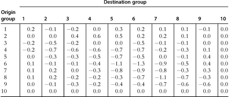
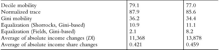
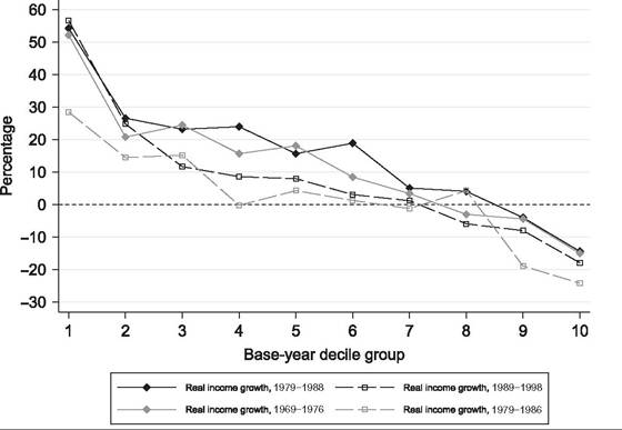
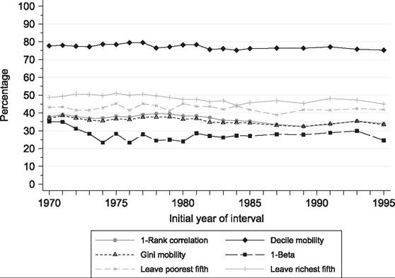
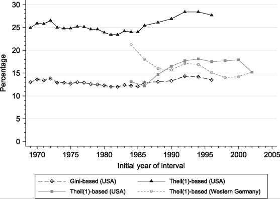
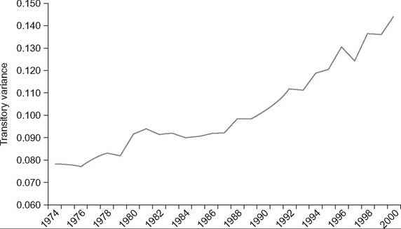
Study Time period covered (Im)mobility measure(s) Remarks Burkhauser and 1983-1988 Shorrocks R First finding that mobility greater in WG than in the USA Burkhauser et al. Year pairs t, t + #964;, Quintile transition Slightly more income (1998) #964; = 1,..., 5, matrices mobility in WG Maasoumi and Trede (2001) 1984-1989 Maasoumi- Greater mobility in WG; statistically significant Gottschalk and 1983, 1993 SWF-based indices WG-USA difference depends on index parameters Schluter and Trede (2003) Year pairs t, t+1 between 1984 and 1992 Shorrocks R WG’s greater mobility arises from greater mobility in low-income ranges Van Kerm (2004) 1985, 1997 Portfolio of indices More income movement in the USA; otherwise varies by index Jenkins and Van Year pairs t, Indices of Reranking and pro- Kerm (2006) t +5: U.S. reranking, progressivity poorness of income growth greater in WG Schluter and Van de Year pairs t, t+1 Index sensitive to U.S. “typically” has gaer (2011) between 1984 and 1992 upward structural mobility more mobility Allanson (2012) Year pairs t, t +5: U.S. 1981-1996, WG 1985-2004 Indices of reranking and structural mobility Reranking and propoorness of income growth greater in WG Demuynck and Van 1984-1985, Indices of USA-WG ranking de gaer (2012) 1996-1997 “inequality- adjusted” income growth depends on weight given low-income-growth individuals Bayaz-Ozturk et al. 5-year windows, Shorrocks R, ratio More mobility in the (2014) alternating years, of permanent to total variance, log incomes USA from around 1990 onward